
Machine Learning 1.0.1. - An overview of Performance Metrics
Machine Learning and how to measure the performance of your model
As mentioned in my previous blogposts, one of the most important steps involved in machine learning is evaluating your machine learning model and finding the best algorithm for your underlying data structure. Normally, the first step after data management is spot checking a variety of different algorithms. But in order to choose your best possible algorithm in order to answer your problem, you need some metrics on which you can compare all of them. This blogpost will give you an overview of some of the mostly used model performance measures in machine learning, with a special focus on classification problems. For a full overview of possible metrics, see here.
Accuracy
![]() Accuracy is the most-cited and easiest to compute and understand measure. It is simply the number of correctly predicted observations over the total number of observations. If your test data consists of 100 individuals, for which you want to make a wage prediction, for example, and your machine learning algorithm got it right for 90 of them, your accuracy score will be 0.9 (or 90). The problem with the accuracy score is that it does not work well under some real world examples, especially when facing Imbalanced Classification Problems. This is due to the fact that simply through predicting the majority class correctly, your model will already report a high accuracy. But this does not really say anything about the importance of your model but instead mirrors the highly skewed class distribution in your data. This is why we need alternative measures we can look at when evaluating our model’s performance.
Accuracy is the most-cited and easiest to compute and understand measure. It is simply the number of correctly predicted observations over the total number of observations. If your test data consists of 100 individuals, for which you want to make a wage prediction, for example, and your machine learning algorithm got it right for 90 of them, your accuracy score will be 0.9 (or 90). The problem with the accuracy score is that it does not work well under some real world examples, especially when facing Imbalanced Classification Problems. This is due to the fact that simply through predicting the majority class correctly, your model will already report a high accuracy. But this does not really say anything about the importance of your model but instead mirrors the highly skewed class distribution in your data. This is why we need alternative measures we can look at when evaluating our model’s performance.
Confusion Matrix
The confusion matrix can help you to identify misclassification and model performance in a fast and visual way. Let’s assume you want to predict if somebody has diabetes or not. A confusion matrix would then look like the below. In the ideal setting, you would only have observations on the diagonal. As soon as there are observations outside the diagonal, your model makes false predictions. Now, in contrast to the accuracy score, the confusion matrix makes a distinction for these false predictions. In the case of our diabetes example, it could be that somebody has diabetes, but our machine learning algorithm classifies him or her as healthy. This is called a False Negative (FN). The other way around, it could be that somebody indeed is healthy but is classified as sick. This is called a False Positive (FP).
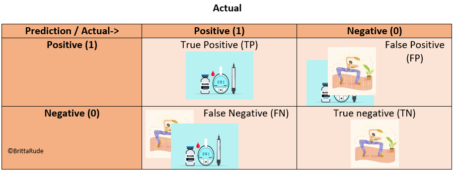
Looking at the table below, accuracy would be equal to the sum of the diagonal divided by the total number of observations in the table, or put differently: Accuracy = (TP + TN)/(TP + TN + FP + FN)
Precision, Recall and the F1-Score
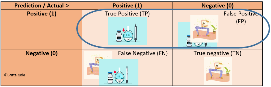
Now, other measures we can look at is precision and recall (Source). Precision only looks at the positive predictions and calculates the share of truly positive values within all positive predictions. Precision is about how many of the diabetes patients we caught through our model (how precise is our model?). Put differently: Precision = TP/(TP + FP)
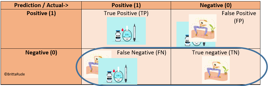
Similarly, Recall only looks at the negative values and calculates the share of truly negative values within all negative predictions. Recall is about how many diabetes patients we missed through our model. This is: Recall = TN/(TN + FN)
Now, the F1-Score combines these two measures into one. More concretely speaking, it is the harmonic average of the Precision and Recall. In the ideal case, the F1 Score is equal to 1.
AUC-ROC Curve
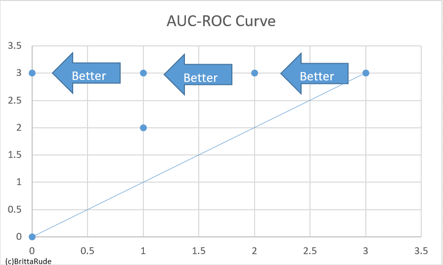
It might be that you are looking at several model specifications of your model. One example is logistic regression. In logistic regressions, you need to determine a threshold for your classification. Your model’s performance might differ, depending on which threshold you use. This is where the ROC Curve can help you (Source). What the ROC (Receiver Operator Characteristic) Curve does is to plot the True Positive Rate (TPR) against the False Positive Rate (FPR). This is much more comfortable than looking at a variety of different confusion matrices, one for each threshold. On the diagonal in the below picture, the TPR is equal to the FPR. As soon as the proportion of true positives is larger than the one of false positives, a data point will lie to the left of our diagonal. In the ideal case, your data point would lie on the Y-Axis (where you plot your TPR). We can also compare different RUC curves (e.g. generated through different algorithm types) to each other through looking at the AUC (Area under the curve). The greater the AUC, the better the algorithm. Note that you can also replace the False Positive Rate with the Precision. This might be suitable in some cases, as for example in the occurrence of a rare disease (Source).
Other evaluation methods
In classification models, you can also look at the Log Loss when evaluating your model. The Log Loss works for binary classification problems (Source). There are other measures to look at, but with the ones mentioned above, you should be covered.
Cross Validation
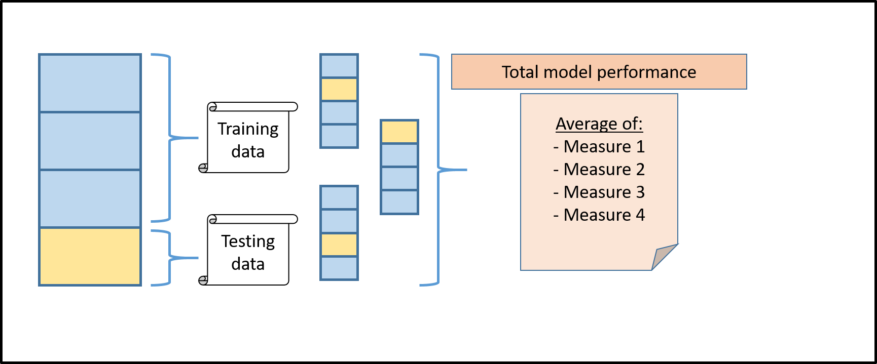
Cross Validation can help us to get an even better understanding of our model’s performance. Instead of just splitting the model once into testing and training data and calculating the accuracy score, for example, we split it many times into different samples and calculate many different accuracy scores. We can then take the average of all these different accuracy scores to calculate our final performance metric. When we train a machine learning algorithm, we typically divide our training data into training and testing. Let’s assume that we have data on 10,000 employees with information about their education, age, occupation and the economic sector they work in. For these 10,000 employees we additionally observe their monthly salary. We have another 10,000 employees for which we observe the same characteristics as above, but lack the information about their wage. What we would like to do is to predict their monthly salary and we can make use of machine learning to do that. We can split our 10,000 employees for which we observe income (our training data) into a subset, for which we train our algorithm, and a subset, for which we make a prediction and then compare it to their actual income (testing data). Let’s assume we take 75 percent of our training data as training and 25 percent as testing data. This would look like the first block in the below image. But how do we know which block is the right one to reserve for testing? Well, there is a simple solution to this. Instead of choosing one, we loop through the overall bar 4 times and each time reserve another of the 3 sub-blocks as testing data (Source). Another question we have to ask ourselves is in how many blocks we would like to divide our data in the first place. Below, we chose to divide it into 4 blocks. This is called Four-Fold Cross Validation.
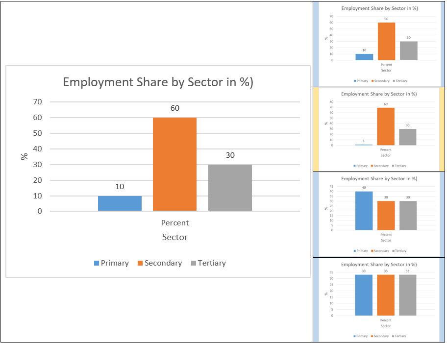
The extreme case of the Four-Fold Cross Validation is dividing our sample by individual observations (in our case employees) and only leaving out one observation for testing. This is referred to as Leave One Out Cross Validation (Source). The most common approach is to divide it into 10 blocks, known as Ten-Fold Cross Validation. A more advanced method of Cross Validation is called Stratified K-Fold Cross-Validation (Source). Stratified K-Fold Cross-Validation makes sense in a lot of real-time applications. Let’s assume that only a small part of our dataset from above works in the primary sector, more concretely speaking, around 10 percent. If we now randomly divide our dataset without taking into consideration this sector share, our model might make biased predictions. One example is the below graph. What we do there is a Four-Fold Cross-Validation. When we take the second block as testing data, a very small share of our subsample works in the primary sector, leading to a very low accuracy of our model in general. This is why we can fix the distribution of workers by sector in each of the 4 blocks. This is then called stratified cross validation leading to models also doing a good job on minority classes.
Through Cross Validation we can compare the performance of different models and choose the best one among all of them. Instead of looking at a single accuracy score, we look at k-different accuracy scores (in the case of Four-Fold Cross Validation at 4 different accuracy scores) and take the mean of all of them (Source). Cross Validation can also help us to find so-called tuning parameters (such as in the case of Ridge or Lasso Regressions) (Source). For an overview of how to implement this in Python, have a look at this video or this one. If you want to understand the difference between cross-validation and test-train-split better have a look at this video.
Ending our tour of performance metrics

This blogpost has presented you with a little tour of different performance metrics. As I mentioned above, due to misclassification problems but also based on other criteria, it is recommended to look at several model performance measures: Confusion Matrix, Precision, Recall, F1 Score, ROC Curve – the list is long! Now, go ahead and cruise some of the different performance measures in order to find the best algorithm for your machine learning model!