Machine Learning 1.0.1. - What is a classifier?

Machine Learning and different types of classifiers

I already mentioned in one of my previous blogposts that there are different types of classifiers we can use to apply machine learning in practice. Many divide these into the following categories: Naïve Bayes Classifier, Regularized Linear Regressions, Support Vector Machines, Decision Trees, k-Nearest Neighbors, as well as Artificial Neural Networks (Source. But what are the differences between all of these? And what is a classifier in the first place, anyhow?

Classifier and Algorithms

So first of all, let’s get back to learning some important terminologies used in the field of machine learning. First of all, what is a classifier? A classifier, as the term might already suggest, classifies information into different categories. One example is our famous newspaper article example, where we try to classify 500 newspaper articles into 5 different categories. Another example is the classification of emails into spam and non-spam (more about this below). It is therefore just one specific type of an algorithm (a sub-category of an algorithm). Algorithms, on the other hand, could have a variety of different goals in mind, such as structure data, parse it, sort it, split it, among many others.

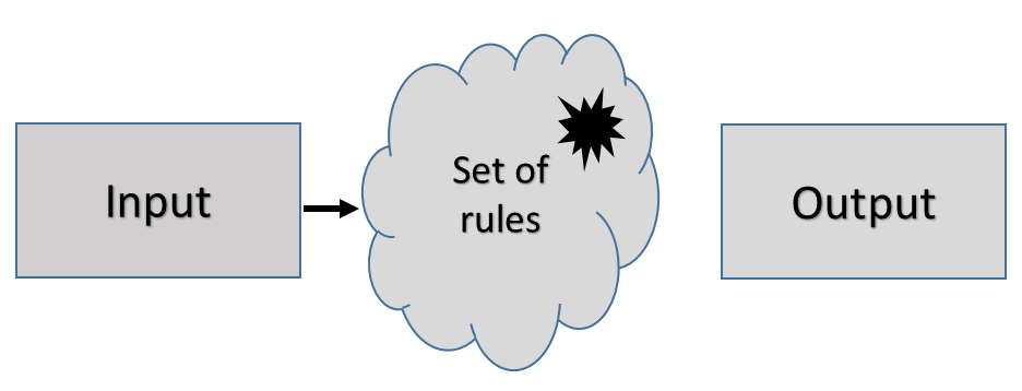
Algorithms, on the other hand, can be seen as a big “set of rules”, which machines follow when solving problems or calculations (Source. An algorithm lives from inputs and rules and creates outputs. For example, we might feed a computer information about the weather during the next 7 days. More concretely speaking, we feed it binary information on if it rains or not (this is our input). We then tell the computer to send us a message to carry an umbrella on the rainy days. We basically tell the computer to apply the following rule: If it rains, send a message saying “Take an umbrella”. This is our rule. The message is then the output generated by the algorithm. We can apply this easily to our newspaper article problem. In this case, our input consists of the 500 newspaper articles and all the words written down there. We then tell the machine to classify an article as “political” as soon as it contains the word “politics” more than 5 times. This is our rule. The algorithm then creates a classification of our newspaper articles, which is the output. This problem then becomes a machine learning algorithm when the data learns from a training dataset (supervised learning) or from itself (unsupervised learning). More concretely speaking, we would

Now, the difference between an algorithm and a model is that the model is the end-result of your algorithm (Source. In other words, through training our algorithm during the training phase of our machine learning exercise, we estimate the parameters behind our machine learning method (Source. For example, it could be that we need a linear or non-linear model, but we do not know this from the beginning. During training, we find the curve which supposedly best fits our data, resulting in our final model. In a second stage we then test the machine learning method. For a more detailed explanation on this, see my previous blogpost.

K-Nearest Neighbor Classification

The KNN Classification is based on the underlying idea that you classify a data point based on its similarity to its direct neighbors. Let’s assume you have a dataset containing a bunch of people’s weight and height and want to classify them into obese and non-obese people. Part of your dataset is already labeled and you can take this dataset to train your classifier. Let’s assume now that you have 5 datapoints: 3 people who are 1,70 Meters tall and weight 60, 65 and 80 kilos, and two people who are 1,50 tall and weight 50 and 70 kilos. We define person 1, 2 and 4 as non-obese and person 3 and 5 are obese. If you now add a sixth, unlabeled data point with the measures 1,60 and 70 kilos and tell our KNN-classifier to label it based on its 5 neighboring values, the algorithm would label it as non-obese. Why? Because the KNN-classifier follows the rule to go for the majority class among all close enough data points. Well, that’s a bummer as we would probably think that somebody who is 1,60 tall and weighs 70 kilos is slightly overweight. Luckily enough, there is a solution to this: Increase the number of data points our new, unlabeled person should be compared to. Let’s assume that there are 3 more obese people with the following measures: 1,50 tall and 100 kilos, 1,55 tall and 100 kilos and 1,80 tall and 100 kilos. Then there is one additional non-obese person, which is 1,80 tall and weighs 80 kilos. If we now tell our algorithm to compare the new, unlabeled data point to all the 9 other people, with the majority being obese, the algorithm will label our new person as obese.

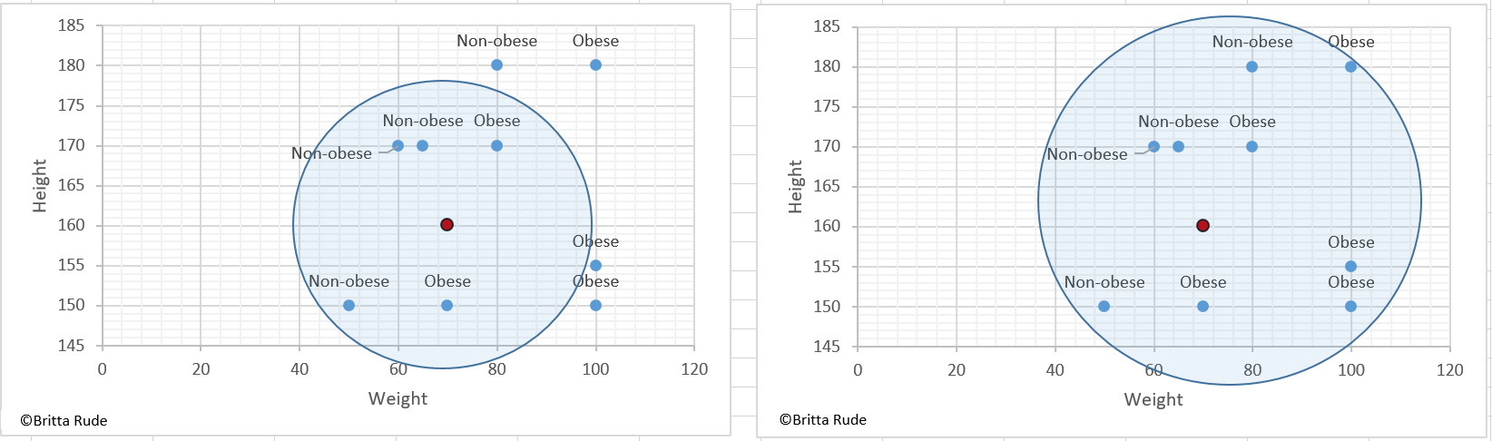
Now, how do we find the nearest neighbors? To identify the data points closest to our unlabeled one, we (or our algorithm) calculated the Euclidean distance. Based on this distance we can then identify the closest Kneighbors we want to compare our unlabeled data to. And how do we choose the right number of neighbors? Well, this is parameter tuning. There are several possibilities how to choose K, but this might be quite random. Some use the square root of the number of observations, for example, as here.

KNN works well when we have labeled data with little noise. The sample should also not be too large (Source). It is not recommended to use KNN with complicated datasets. In general, the KNN classifier might take quite some time to run, especially with a larger number of neighbors.

Decision Tree

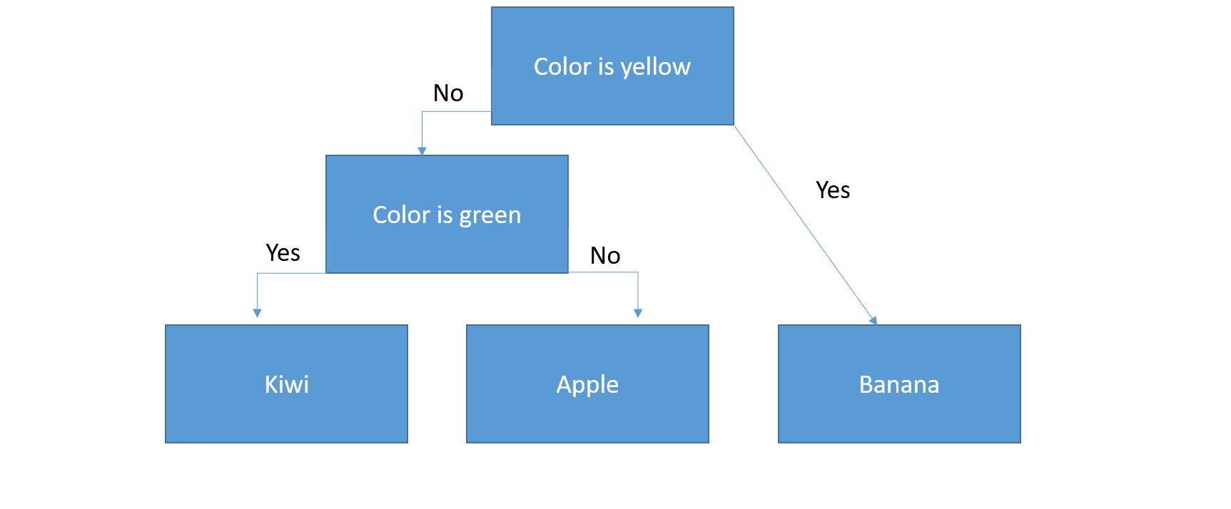
Decision trees belong to the category of supervised learning (Source). They also go by the name CART or Classification And Regression Trees. One of its most known and applied variations is called Random Forest. A decision tree consists of nodes, representing respective input variables, and leaf nodes with the output variable. Let’s assume you have three fruits, an apple, banana and kiwi, and want to teach your machine to distinguish between them based on their respective colors. The set of rules that we can deduct from our tree goes as follows:

If Color=Yellow Then Banana

If Color!=Yellow and Diameter<2 Then Kiwi

If Color!=Yellow and Diameter>2 Then Apple

The example above shows that a decision tree consists of branches. At each branch, we make a decision. The so-called decision can also be a reaction or occurrence (Source). The last stage on the bottom of a decision tree is called the leaf note and contains the final classification of the exercise. Similarly, the first stage at the top of the tree is called root node. A tree’s depth is the number of stages (layers) and a tree’s leaves is the number of categories (boxes) in the root node (bottom layer).

When evaluating decision trees, we need to be aware of a number of other concepts. First, entropy: Entropy measures the degree of randomness or unpredictability in a dataset. Then there is information gain. Information gain measures the decrease in entropy through splitting our dataset. A decision tree algorithm is nothing more or less than the solution to another optimization problem. What we try to do is to minimize our famous loss function (or cost function), which in this case is the entropy. Or, put differently, we try to maximize the information gain. For the formula behind the entropy, have a look at this video.

So how can we apply these decision trees in Machine Learning? Let’s assume you want to predict if somebody earns more than 100,000 US-Dollar, based on the company, a person’s job title as well as degree, such as in this example. In the pre-machine times, we would conduct this manually through building a decision tree by hand. Probably we would start by the company, then continue to the job position and lastly the degree. This might be still quite simple, but in many cases you might face hundreds of attributes and thousands of employees. Doing the task manually would therefore become quite challenging and take a crazy amount of time. Now, the good thing is that we can led machines do the needy, greedy work for us. We therefore, similar to all the other machine learning examples, train our machine on training data, meaning that we have a dataset, for which we already observe the salary for each employee.

You feed the algorithm some pre-defined parameters, such as the maximum number of layers (depth) and the minimum number of leaves (final categories). This is required as the algorithm needs to know when to stop. You can determine the optimal number of splits through pruning. The underlying idea behind pruning is that you, after every additional split, ask yourself if the split was really necessary (has led to any considerable improvements, or a drop in the cost function). A more sophisticated method of pruning goes under the name cost complexity pruning and takes into account a learning parameter for the decision to remove nodes or not. We then run the algorithm on our training data (let’s say, 30 percent of our pre-labeled dataset) and predict the salary on our testing data (the remaining 70 percent of our pre-labeled dataset). We can evaluate the model’s performance through our famous accuracy. If we like what we see, we can then make a prediction on new, unseen and unlabeled data.

Decision trees are easy to visualize and interpret. We also have to do little data preparation when working with decision trees and they perform well under non-linear parameters. Sadly, decision trees often suffer from overfitting and high variance. Additionally, in the case of low bias, the model might not work well on unseen data. For the Python codes behind all of this, have a look at this video.

Naïve Bayes classifier

The Naïve Bayes classifier is a conditional probability model. This model is based on the independence assumption, meaning that it assumes independence in the explanatory variables (features). Let’s assume you have a sample of people with information about height, weight and foot size. You want to classify this sample into male and female people. The Naïve Bayes classifier assumes that each of the 3 characteristics contribute equally to one’s gender, abstracting of possible correlations between these. In the case of text data, the algorithm abstracts from any relationship between different words or the significance of the words’ ordering. The Naïve Bayes classifier then applies a decision rule based on probability. More concretely speaking, it first calculates the conditional probability, based on Bayes’ theorem, and then maximizes this conditional probability.

To illustrate this, let’s have a look at a concrete example, the classification of emails into spam and non-spam. We have a training data set of emails, which we hand-coded into spam and non-spam. This training data consists of 20,000 words. 6,000 of these words belong to spam and the remaining 14,000 to non-spam emails. We can then, for every word in these emails, calculate its probability to belong to spam or non-spam emails. Let’s take the word “million” and assume that it appears 100 times in the subset of spam emails and 10 times in the subset of non-spam emails. Its probability to be spam is then 100/6,000. Similary, its probability to be non-spam is 10/14,000. Its likelihood ratio to be spam is then (100/6,000) / (10/14,000) = 23.33. The Bayes’ theorem calculated the conditional probability through multiplying the a-priory probability by the likelihood ratio. Let’s assume that we know that half of emails are spam and half are non-spam. The A-priori probability is 0.5 and our likelihood ratios are calculated as shown in the example above. For a detailed overview of what an A-priority probability is, see here. For a practical application, follow this code.

The problem with the Naïve Bayes classifier is its independence assumption. Assuming that the all predictors (or features) are independent is highly unlikely in real life. Additionally, the algorithm suffers from a zero-frequency problem. Let’s say the word “sunny” did not appear in your training data, but does appear in your testing data. The Naïve Bayes classifier will assign a zero probability to all of these cases (Source. It simply ignores unknown words (Source and cannot classify unseen, new words. One can solve this through smoothing techniques, such as the Laplace estimation. For the underlying rational see this discussion. And for a summary of the Pros and Cons of this model, see here. Naïve Bayes is great as it is very simple and easy to implement, needs less training data, is relatively fast and highly scalable, can deal both with continuous and categorical variables and is not sensitive to irrelevant features (Source).

Regularized linear and logistic models

Regularized linear models are one of the most popular algorithms for supervised learning tasks. In my previous blogpost I gave you a little reminder of simple linear regressions and OLS (ordinary least square). To review the basic mathematical annotations behind this, see here. The problem with this is that it does not work in some cases. One problem is multicollinearity. Multicollinearity is when our explanatory variables depend on each other (have some form of relationship with each other). Remember the example above on height, weight and foot size? My weight definitely depends on my height, so assuming that they independently influence the gender of a person might be a strong assumption and not hold in reality. The other problem is that now, with big data, we often have cases where we have more explanatory variables than data points. Let’s take our typical example of 500 newspaper articles we would like to classify into 5 different categories. My categorization depends on the text included in these newspaper articles. I might have many more words than data points (500 newspaper articles). In this case the number of independent variables (words) is larger than the number of observations and OLS is not valid anymore. The solution to the optimization problem might not be unique anymore, or might be subject to overfitting. You can solve this via only selecting the most important features (explanatory variables), through reducing the dimensionality of the dataset (e.g. through stemming in the case of text data), or via regularization. Regularization means adding a penalty to the loss function (in the case of OLS the loss function is the sum of squared errors). Depending on how the regularizing term looks like, we call these new functions Ridge Regressions, Lasso Regressions, or Elastic Nets. Let’s have a look at all three of them.

To start with, let’s remind ourselves of an important concept, the bias-variance tradeoff. To remind ourselves what this is about, let’s revisit a practical example. Let’s assume your weight is 60.34 kg. Let’s now imagine that we have to choose between 4 different balances. To test their accuracy, we weight ourselves on each of the three balanced three times. You note down the following results:

• Balance 1: 60.2, 60.5, 60.4, 60.4: This balance has low variance (deviations) and low bias (gives the correct mean, which is 60.34 kg).
• Balance 2: 58.2, 57.9, 58.0, 59.0: This balance has low variance (deviations), but a bias (the average is 58.3 kg and too low).
• Balance 3: 55.9, 65.8, 57.2, 63.2: This balance has high variance (deviations), but low bias (the average is 60.5 and close to our actual weight).

Now, you might obviously want to choose Balance 1. The thing is that this option does not exist under collinearity. You need to choose between having a bias (Balance 2, or Ridge Regressions), or a high variance (Balance 3, or OLS Regression). Another way to embark this is through thinking about the limitations of data analysis in the first place. Let’s go back to our actual weight. What is our actual weight, in the end? Should we weight ourselves first thing in the morning, before having a glass of water, or afterwards? Before or after having breakfast? Before going to the toilet, or afterwards? Before or after going to the gym and sweating out half a liter of liquids? So what you might actually look for is some kind of super-balance, which takes all of these factors playing a role in your final weight into account. This new super-balance would maybe draw from information such as the timing of the day and your weight from past days. If the super-balance notices that your weight at 6 am in the morning is 0.5 kilos lower than the average weight of past days around 10 am, and 0.5 kilos heavier at 7 pm, it might guess that his has to do with your clothing, or water and food consumption, and shrink the observations from 6 am and 7 pm towards the observed average from past days. We will then have less variance, but also a bias, as we might not get exactly to the average, or report actual weight changes in delays. This is exactly the underlying concept of ridge regressions. Do you remember our example on education and wages and the fact that there were some employees which had surprisingly high wages for their education level (so-called outliers). Well, ridge regression would add some artificial employees, which would cancel out these outliers.

This is how we avoid overfitting. In mathematical terms this means adding a regularization penalty to our loss function (Source). In the case of OLS we would add a penalty to the sum of squared errors. The penalty consists of a tuning parameter (lambda) and the penalty (in the case of ridge often referred to as L2). L2 is a linear function of the squared coefficients forming part of the model. Importantly, in ridge regressions, we only shrink our parameter coefficients but do not fully kick them out (Source). This is why all independent variables form part of the model. This is the main difference to lasso regressions, which we will look at next.

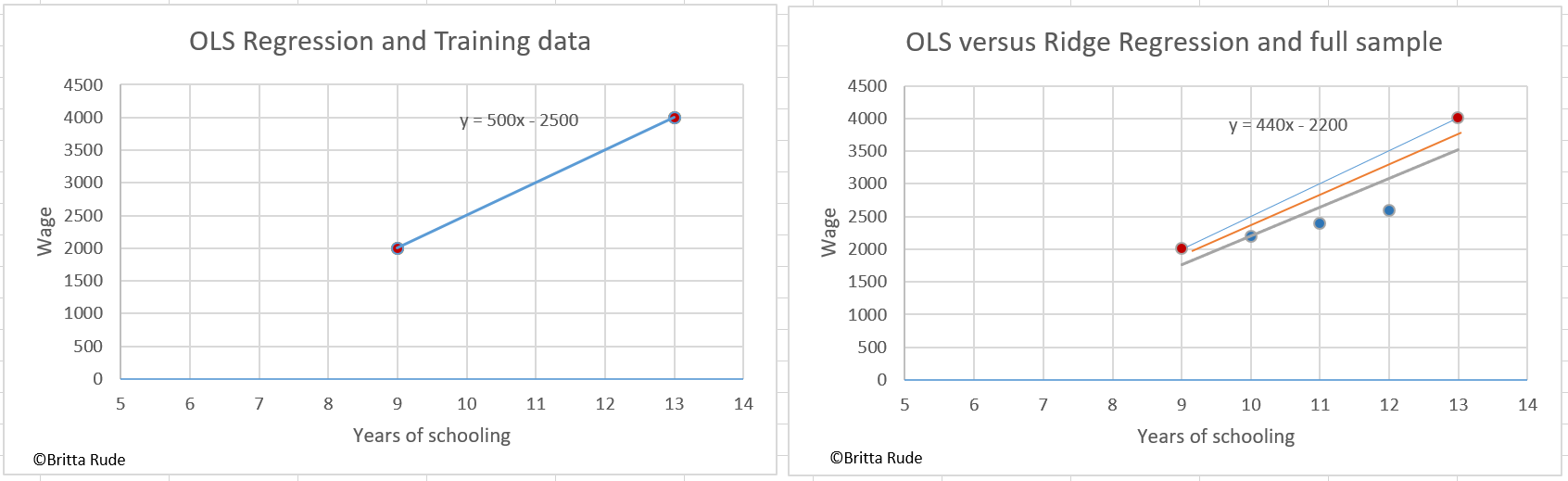
Well, this sounds all very abstract, so let’s have a look at a concrete example. Let’s assume we would like to predict the wages of people based on their years of education. Let’s assume that our training data only consists of two data points: One employee with 10 years of education and earning 2000 currencies and another one with 13 years of education and earning 4000 currencies. OLS from this equation would assume that the effect of education on wages is 500. Looking at our graph below, when adding the testing data, which consists of an additional 3 employees, this is an overestimation. OLS overfitted the highest salary, which was actually some kind of outlier. The actual relation is much lower with 440. Ridge (the orange line in the right graph) tries to account for this through introducing a slight bias, but decreasing the variance and the risk of overfitting. If the concept is not yet clear, have a look at this video, which gives a very clear explanation. On a practical example of how to apply ridge with Python, have a look here.

Lasso works similarly to ridge regressions, but instead of using the L2 penalization, it applies an L1 penalization. This means that it adds a penalization which is equal to the weighted sum of the models coefficients (Source). This means that, different from ridge, some of the coefficients will be zero, leading to what is known under the term feature selection. The model will therefore be simpler and include less independent variables. For the mathematical details behind this, see here. For a practical application of Lasso in Python, see here. So now that we know what Ridge and Lasso look like, we can have a look at their common child, the Elastic Net. The elastic net combines the penalty from ridge and lasso through including them both and weighting them by an additional parameter (alpha). Here you can see how this looks formula-wise and this is a nice practical example in Python (for a video tutorial see this example by Simplilearn.

By the way, the tuning parameter (lambda) is quite important in linear regressions. In Lasso, a tuning parameter of zero would be equal to an OLS regression while a lambda of infinite value would be equal to a model consisting of an intercept only. We can find the optimal tuning parameter through Cross Validation (CV) or looking at other parameters, such as AIC (Akaike’s Information Criterion), and BIC (Bayesian Information Criterion). The problem with these linear regressions is that they are often outperformed by more complex algorithms, leading to better predictions. Still, they are easier to understand and interpret. When should we use Lasso and when Ridge? The rule of thumb is to use Ridge Regularization in cases where you have many variables with relatively little data and to use Lasso Regularization in cases where you have fewer variables (Source).

Support Vector Machine

I already talked about SVM in one of my previous blogposts. Just to give you a little reminder, the underlying idea behind SVM is to separate data points into different classes through drawing a line which maximizes the space between them, only that in SVM we do not approach this via the line but a hyperplane and support vectors. You might remember that the dimension of the hyperplane depends on the number of features. The SVM works well on high-dimensional data, sparse document vectors and addresses overfitting and bias problems (Source). For a nice example see this video.

Random Forests

Random Forests are one of the most advanced algorithms and form part of the so-called ensemble classifiers. These are classifiers, which combine the estimations of several individual estimators to make a better prediction. More specifically, they form part of the group of Parallel Ensemble Methods (more about this later). Random Forests are used in a variety of applications, such as remote sensing, multiclass object detection as well as game console technologies (Source). What the random forest does is to estimate several individual decision trees and then take the majority vote as the final decision. Let’s take the example of below. You want to predict if an animal is a cat or a lamb. You do 3 different decision trees, of which 2 tell you that it is a cat while one tells you that it is a lamb. The Random Forest algorithm looks at all trees, the so-called forest, and takes the majority vote as the final outcome, in this case, the cat.

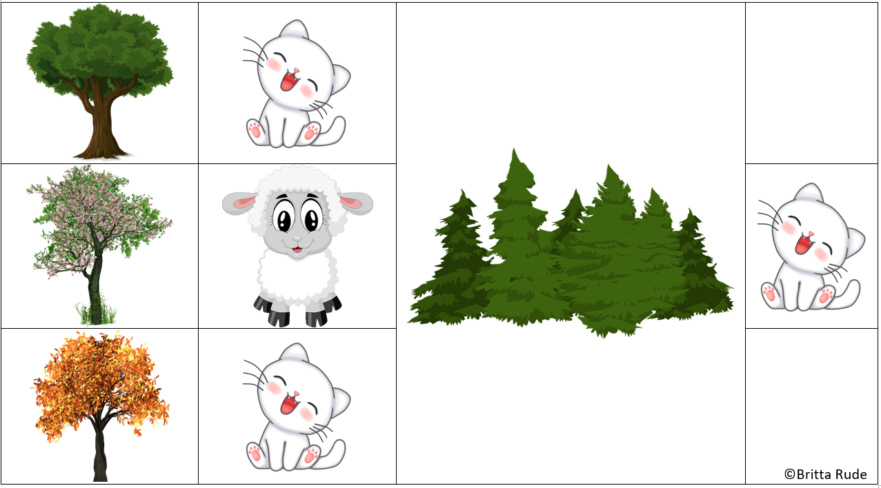
But where do these different predictions come from in the first place? Well, the outcome of the tree depends on the ordering of the decision parameters. Below there are 3 different trees with different outcome. Now, let’s assume you have a white, big dog. The first tree will tell you that the animal is a lamb, the second one that it is a cat and the third one that it is a lamb. So the final decision of the forest tree would classify the white, big dig as a lamb.

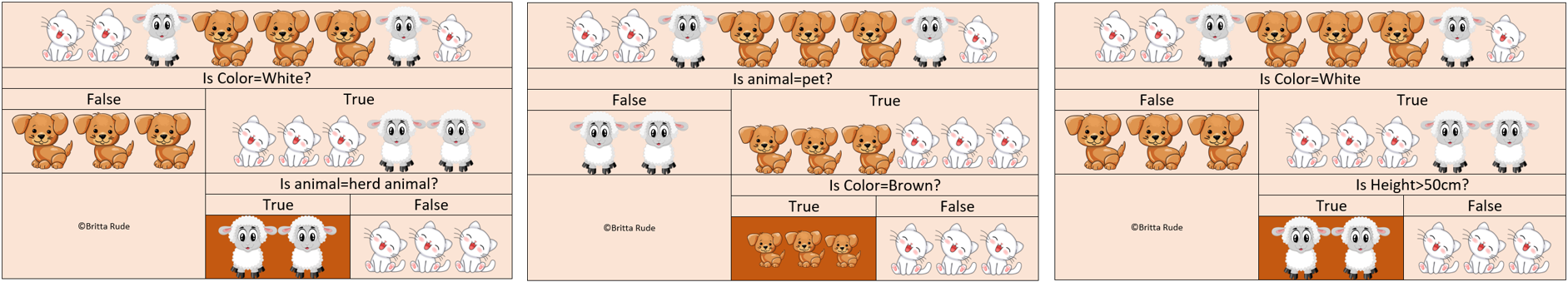
As you can see in the picture above, the 3 trees are generated in parallel. This is why Random Forests form part of the Parallel Ensemble Methods and not the Sequential Ensemble Methods (more about this later) (Source). Through combining several trees instead of just looking at one tree, the overall model’s prediction will be more accurate and more robust.

Summing up

Well, as you have seen there is no shortage of classifiers out there! When trying to solve a classification problem, you can start by spot-checking some of those and comparing their performance. Or you can take a step back, think about the structure of your data and decide about which type of classifier will work best for the kind or problem you are facing! Logistic Regressions are great for binominal outcomes, K-Nearest Neighbors works well for pattern recognition or data mining, SVM might be the best model when working with high-dimensional data and Decision Trees should be used for decision analysis (Source). All of the above algorithms face their limitations and disadvantages. While Logistic Regression relies on a high representability of data, KNN does not work well with high-dimensional data. SVM and Decision Trees, on the other hand, do not work well with large datasets and datasets with a lot of noise. There are some methods and measures you can look at to detect the best possible classifier among all the ones you are looking at, but that is food for a future blogpost. For now, have fun experimenting with some ML classifiers!