
Machine Learning 1.0.1. - Supervised Learning
Machine Learning 1.0.1. – What is Supervised Learning? Machine Learning is becoming more and more present in Data Science, but also other fields and areas. But what is that, actually – Machine Learning? The name already speaks for itself: We teach machines to learn on their own. Quite abstract, you think? Not at all! Let’s have a look at a concrete example of Machine Learning, which is Supervised Learning. In this blog post we will look at some important concepts of Machine Learning, such as Over- and Underfitting, Loss Functions, Optimizers, Gradient Descents, the Learning Rate and Regularization.
A simple example: Classifying a large number of newspaper articles into 5 different categories

Let’s assume you have a set of newspaper articles which you want to classify into 5 different categories: Politics, Economics, Sports, Entertainment and Others. If you have 5 different newspaper you might still be able to do this on your own. But what about 500 newspaper articles? It might be quite tedious and take a lot of time to do this. And here is where machine learning can help. Instead of looking at each 500 newspaper article one by one you can just do this exercise for a small subset of newspapers (let’s say 5 percent, which would be 50 newspaper articles). You then feed this information to a machine and train the model based on this 50 newspaper articles and the respective categories. On the basis of this information, the model will then learn to code the rest of the 450 newspaper articles. You can even evaluate the effectiveness of your trained model, but more about this later. First, let’s try to understand a bit better how this model training exactly looks like.
What is behind the training of a machine? An intuitive comparison
We can train the model through making predictions based on the text which is included in each article. The variable (information) we would like to predict is the category (classification). Economists often call this an outcome variable. The information (variable) we use to explain this outcome variable is our article text. The informative variable also often goes by the name explanatory variable. Many of you might remember simple linear mathematical regressions from high-school (Y = a + X * b). Simple examples for regressions are for example the effect of education on wages. You can take a number of employees, ask them about their years of education as well as their wages and from there infer a relationship between wages and education. Typically, this relationship would be positive (although probably not linear). You might find out that one year of education leads to an increase in wages of 10 percent (I am just making this up). You can then even take this information and predict the wages for a number of employees, for which you only observe the years of education, but not wages. This would of course be highly oversimplified, but I am just trying to explain the underlying intuition here. So, in the case of our example, we try to do something similar, only that now we replace the years of education by text and the wages by our 5 categories.
Finding the right algorithm
There are a variety of different possibilities to run the math behind supervised learning algorithms. The magic behind machine learning is its generalization. Put differently, how well do the concepts learned by the model from hand-coded data apply to new data? For example, the machine might learn from my hand-coded data that as soon as the word “politics” appears more than 5 times, a newspaper article belongs to the category “politics”. But the unseen data might contain new words, which were not included in the 50 articles we hand-coded before (e.g. politicians). This can lead to errors in the classification of the remaining 450 newspaper articles. What do we have to have in mind when choosing the right algorithm for our classification?
Over- and underfitting problems
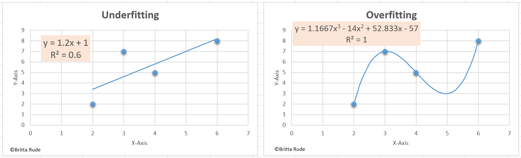
Underfitting is easy to understand and detect: Our model simply does not learn well enough from the training data and makes false predictions within the training data and therefore also outside of the training data (Source). For example, we might assume that the relationship between wages and education is linear. In reality, this might not be the case. We can then try to correct the model by assuming a non-linear relationship between both variables. Overfitting is less easy to understand and detect: The model copies the algorithm too well. To understand this, let’s go back to our employee database (Source). Let’s assume that there are some employees with immensely high wages in our sample. This might just be a coincidence as we did not do a good job when drawing a random sample. Our model could then misunderstand this information and take this information into account when deriving the relationship between wages and education. This, on the other hand, might then lead again to false predictions for new employees, for which we just have information about their level of education. For a concrete mathematical example, have a look here.
This is why, for machine learning, we need more complex solutions for our predictions than a simple linear regression. There are a variety of different methods to do that: Regularized regressions, Naïve Bayes, Support Vector Machines or Ensemble classifiers. They are all algorithms, similar to our linear regression, but more efficient and much more powerful. Let’s have a look at one of them, the Support Vector Machines algorithm.
What is a Support Vector Machine?

SVM is known for its high accuracy with relatively low computational power. What SVM does is to classify our data in a sense that it maximizes the distance between data points belonging to each class. SVM approaches this problem through hyperplanes. A hyperplane is a decision boundary which helps to separate the different data points. The dimensionality of this hyperplane (e.g. 2-dimensional or 3-dimensional, or many more) depends on the number of features (e.g. document articles) you feed into the model. We can maximize the distance between data points of each class through this hyperplanes via support vectors.
The Loss Function
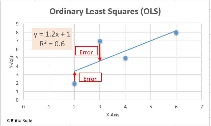
Well, now we might have gotten in a bit of an abstract sphere here. Remember our wage and education example? When we estimate the relationship, we try to minimize the error in this estimation, right? Have a look at the Figure below to understand it better. What we try to find is an optimal solution through which we minimize the errors (the red bars). In order to avoid a canceling out of positive and negative errors, we take the square of those. This is what we often call Ordinary Least Squares (OLS). So what we have here is a minimization problem. In machine learning, we try to do something similar. More concretely speaking, our goal is to find a function which models our data well (which conducts a correct prediction on the new data, in our case, the 450 newspaper articles). In machine learning, we evaluate this through the so-called loss function. Put differently, the loss function is the function which measures how well our chosen algorithm models our data. The worse the prediction, the higher the total loss. Let’s assume that our model predicts that an employee with 12 years of schooling earns 2,000 Euros per month. If this person in reality earns 1,800 Euros we are off by 200. The same for an employee with 12 years of schooling earning 2,200 Euros. We then aggregate all these false predictions to calculate our overall loss.
The loss function can take several different forms. In OLS, we calculate the Mean Squared Error (MSE), for example. In MSE we simply take the difference between all of our predictions and all of our real data points (in our above example, wages), square them and then take the average. Another example is the Likelihood Loss function, which can be applied when predicting probabilities. Let’s assume we want to predict the probability that it rains during the next 4 days. If our algorithm tells us that the probability for Monday is 20 percent, Tuesday 40 percent, Wednesday 60 percent and Thursday 80 percent but it then rains on every single day (the actual probability is 100 percent for each day), we would take the deviation for each day (80 percent, 60 percent, 40 percent and 20 percent) and multiply them by each other: 80*60*40*20. There are other options, such as the Log Loss Function, which is similar to the Likelihood Loss function, but penalizes those terms which are very wrong by more. So now that we know that our end goal is to minimize this Loss Function (no matter which form it takes), we can use this to construct our algorithm in the first place. What we do is to minimize the loss function (our false predictions) through an optimizer. Similar to OLS, we have an optimization problem here. We try to minimize something.
The Optimizer

There are a variety of different optimizers available to find the best method for making predictions on new data. What the optimizer does is to replace parameter after parameter in our model, check the loss function, and stop when it has found the best possible solution with the lowest possible loss. To get a better grasp of how this works, let’s assume that we are blind, for a moment, standing close to a traffic light. In Germany, many traffic lights make sounds when they jump to green, in order to make crossing possible for blind people. So, you might not see where you have to go and when the light turns green, but you for sure will know if you walk into the right or wrong direction, based on the sound of the traffic light. The closer you get, the louder the sound of the traffic light. In machine learning, the traffic light is the loss function, and the blind person our optimizer. The loss function will guide the optimizer to walk into the right direction, towards our optimal solution.
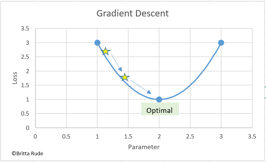
Let’s have a look at a concrete example: The Gradient Descent. What the Gradient Descent does is to change our parameters (e.g. the strength of relationship between education and wages) by a little and have a look at what this does to the loss (accuracy of the model). Based on this information (which is called the Gradient), the Gradient Descent then adjusts the parameters (in machine learning also sometimes called weights) until getting to the lowest point of a loss function. The Gradient is nothing more and less than a partial derivative, and therefore a tiny little change. By the way, we do not have to calculate the gradients for our entire training data (e.g. the 45 newspaper articles we hand-coded). We can also just calculate it for a subset (let’s say 30 newspaper articles). This goes by the name Stochastic Gradient Descent.
The Learning Rate
One downside with optimizers is that you might get to a “false optimal”. Let’s go back to our blind person. Instead of just crossing one traffic light to get to our final destination, we now have to cross 3 traffic lights. But we do not know this beforehand and might therefore stay at traffic light 1 instead of crossing all 3 traffic lights. We might therefore never get to our final destination, in the case of optimizers, the point where we minimize our loss function. Luckily, there is a method to avoid this, which is the learning rate. Let’s assume that we now have 4 traffic lights which are directly next to each other. If we walk extremely fast, we might not be able to distinguish one traffic lights’ sound from another anymore and just walk straight over them. We then miss our final location which was located at traffic light 3. If we walk too slow, on the other hand, we might never become aware of the fact that there are actually several traffic lights and that we should cross more than one. We therefore have to find the right walking pace to get to our final destination. In the case of our optimizer, we have to find the right gradient (the right magnitude) through which we change our parameter. If our rate of change is too large or too small, we might miss the optima or get stuck at false local minima.
Regularization
I already talked about the problem of Overfitting in this blogpost. Overfitting actually evolves when one parameter takes too much weight in our formula (function). We can solve this by adding a so-called penalty term to the error function (loss function). This is called Regularization. We penalize those terms, which are extremely large. Remember our employee with an extremely high salary for their education level? This is an outlier, or noise, in our dataset. Regularization would penalize this employee and therefore avoid that they take too much influence on our underlying estimation between education and wages.
Back to SVM
Great! Now back to our SVM. In SVM, our loss function is called hinge loss. This loss function helps us to maximize the margin between our data points and hyperplane. For each predicted and actual value (e.g. each predicted and actual employee wage) we calculate the loss (the prediction error). We then add a regularization parameter to the loss function in order to control for overfitting. Next, we take partial derivatives of this function and derive our gradients. Through these gradients we then get to our optimal solution and the best possible prediction of our 450 not-coded newspaper articles.
Wrapping it up!
So, Machine Learning – in this case, Supervised Learning – can help us to conduct otherwise tedious and time-costly tasks, such as the classification of 500 newspaper articles. By hand-coding a subset of our dataset (as for example 50 newspaper articles) we can train the machine to code the rest of the 450 newspaper articles. Our goal is to design an algorithm which performs well on the unseen data (the 450 remaining newspaper articles). We do this through the application of an optimizer and a loss function. We use our optimizer to minimize our loss (the prediction errors). One example is the Gradient Descent. The Learning Rate can help us with that! Do not forget to introduce a penalty term and regulate your loss function. This is how you avoid overfitting and control for the noise in your training data.