Forecasting with Python - and how Machine Learning can help

The art of Forecasting with Python

Often we need to make predictions about the future. In the private sector we would like to know how certain markets relevant to our businesses develop in the next months or years to make the right investment decisions, and in the public sector we would like to know when to expect the next episode of economic decline. There is an entire art behind the development of future forecasts.

Economists have tried to improve their predictions through modeling for decades now, but models still tend to fail, and there is a lot of room for improvement. Lately, machine learning has fed into the art of forecasting. This blog post gives an example of how to build a forecasting model in Python. For that, let’s assume I am interested in the development of global wood demand during the next 10 years. Let’s rely on data published by FAOSTAT for that purpose. You can find the data on this link. Let’s download the import quantity data for all years, items and countries and assume that it is a good proxy for global wood demand.

Let’s know prepare the dataset for our purpose through grouping it by year.

dataset = pd.read_excel('C:/Users/FAOSTAT_data_11-13-2020.xls')

demand = dataset[dataset["Element"]=="Import Quantity"]
demand = demand[["Area", "Element", "Item", "Year", "Value"]]
demand = demand.groupby("Year").sum().reset_index()
demand.head()

To do forecasts in Python, we need to create a time series. A time-series is a data sequence which has timely data points, e.g. one data point for each day, month or year. In Python, we indicate a time series through passing a date-type variable to the index:

demand["Year_str"] = demand["Year"].astype(str)
demand['Year_date'] = demand['Year_str'] + "-01-01"
demand["Year_date"] = pd.to_datetime(demand["Year_date"])
demand = demand.set_index("Year_date")
demand.dtypes

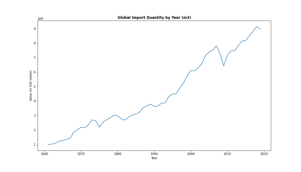
Let’s plot our graph now to see how the time series looks over time:

plt.figure(figsize=(14,8))
ax = sns.lineplot(data=demand, x="Year", y="Value")
plt.title('Global Import Quantity by Year (m3)', fontsize=12, fontweight='bold')
plt.ylabel("Value (in 100 million")

Global Wood Demand

So we are all set up now to do our forecast. But first, let’s have a look at which economic model we will use to do our forecast.

The Theory behind the Practice - SARIMAX Forecasting

There are a lot of ways to do forecasts, and a lot of different models which we can apply. In this blogpost I will just focus on one particular model, called the SARIMAX model, or Seasonal Autoregressive Integrated Moving Average with Explanatory Variable Model. Let’s look at this one by one:

Seasonal (S): Seasonal means that our data has a seasonal trend, as for example business cycles, which occur over and over again at a certain point in time.
Autoregressive (AR): Autoregressive is a time series that depends on past values, that is, you autoregresse a future value on its past values. You define the number of past values you want to consider for your forecast, the so called order of your AR term through the parameter p.
Intgrated Moving Average (IMA): The integrated moving average part of an SARIMAX model comes from the fact that you take into account the past forecasting errors to correct your future forecasts. What does this means? Let’s assume you have a time-series of 4 values, April, May, June and July. Now - as a first step, you predict the value in June based on the observed predictions in April and May. You then compare your actual value in June with the forecasted value, and take the deviation into account to make your prediction for July. You define the number of Moving Average terms you want to include into your model through the parameter q.
Explanatory Variable (X): This means that the evolution of the time series of interest does not only depend on itself, but also on external variables. Wood demand, for example, might depend on how the economy in general evolves, and on population growth. This is what marks the difference between a univariate and a multivariate forecasting model.

Making your data stationary

But before starting to build or optimal forecasting model, we need to make our time-series stationary. Stationary means that the statistical properties like mean, variance, and autocorrelation of your dataset stay the same over time. This can be achieved through differencing our time series. Sometimes it is sufficient to difference our data once, but sometimes it might be necessary to difference it two, three or even more times. This you define through the parameter d.

So, let’s investigate if our data is stationary. There is a simple test for this, which is called the Augmented Dickey-Fuller Test. In Pyhton, there is a simple code for this:

from statsmodels.tsa.stattools import adfuller
from numpy import log
result = adfuller(demand.Value.dropna())
print('ADF Statistic: %f' % result[0]) #ADF Statistic: 0.608666
print('p-value: %f' % result[1]) #p-value: 0.987827 - greater than significance level

Looking at the AFD test, we can see that the data is not stationary.

As an alternative, we can plot the rolling statistics, that is, the mean and standard deviation over time:

 def test_stationarity(timeseries, title):
    
    #Determing rolling statistics
    rolmean = pd.Series(timeseries).rolling(window=12).mean() 
    rolstd = pd.Series(timeseries).rolling(window=12).std()
    
    fig, ax = plt.subplots(figsize=(16, 4))
    ax.plot(timeseries, label= title)
    ax.plot(rolmean, label='rolling mean');
    ax.plot(rolstd, label='rolling std (x10)');
    ax.legend() 
    
pd.options.display.float_format = '{:.8f}'.format
test_stationarity(demand.Value,'raw data')

We can take care of the non-stationary through detrending, or differencing. Detrending removes the underlying trend below your data, e.g. an ever increasing time-series. Differencing removes cyclical or seasonal patterns. You can alos combine both. We could do this manually now, but our optimal forecasting model will take care of both automatically, so no need to do this now.

Get prepared for some Machine Learning - Testing and Training Datasets

How can we get to our optimal forecasting model? We need to be able to evaluate its performance. And therefore we need to create a testing and a training dataset. So let’s split our dataset. In our case we will reserve all values after 2000 to evaluate our model. This is consistent with splitting the testing and training dataset by a proportion of 75 to 25.

train = demand.query("Year<2000")
test = demand.query("Year>2000")
y_train = train.Value
y_test = test.Value

Create your optimal SARIMAX Forecasting Model

I already talked about the different parameters of the SARIMAX model above. This is why you will often find the following connotation of the SARIMAX model: SARIMA(p,d,q)(P,D,Q). Python can easily help us with finding the optimal parameters (p,d,q) as well as (P,D,Q) through comparing all possible combinations of these parameters and choose the model with the least forecasting error, applying a criterion that is called the AIC (Akaike Information Criterion). The AIC measures how well the a model fits the actual data and also accounts for the complexity of the model. Python picks the model with the lowest AIC for us:

from statsmodels.tsa.arima_model import ARIMA
import pmdarima as pm
smodel = pm.auto_arima(demand.Value, start_p=1, start_q=1,
                         test='adf',
                         max_p=3, max_q=3, m=10,
                         start_P=0, seasonal=True,
                         d=None, D=1, trace=True,
                         error_action='ignore',  
                         suppress_warnings=True, 
                         stepwise=True)

smodel.summary()

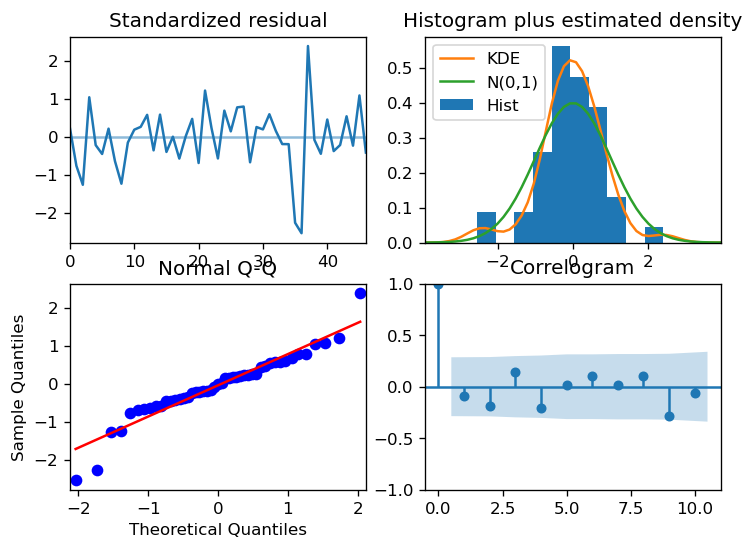
We can then check the robustness of our models through looking at the residuals:

model.plot_diagnostics(figsize=(7,5))
plt.show()

Diagnostics

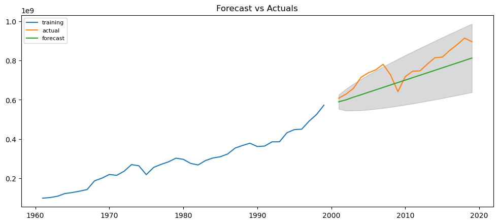
What is actually happening behind the scenes of the auto_arima is a form of machine learning. The model trains the part of the data which we reserved as our training dataset, and then compares it the testing values. Below we can do this exercise manually for an ARIMA(1,1,1) model:

# Build Model
# model = ARIMA(train, order=(3,2,1))  
model = ARIMA(y_train, order=(1, 1, 1))  
fitted = model.fit(disp=-1)  

# Forecast
fc, se, conf = fitted.forecast(19, alpha=0.05)  # 95% conf

# Make as pandas series
fc_series = pd.Series(fc, index=test.index)
lower_series = pd.Series(conf[:, 0], index=test.index)
upper_series = pd.Series(conf[:, 1], index=test.index)

# Plot
plt.figure(figsize=(12,5), dpi=100)
plt.plot(y_train, label='training')
plt.plot(y_test, label='actual')
plt.plot(fc_series, label='forecast')
plt.fill_between(lower_series.index, lower_series, upper_series, 
                 color='k', alpha=.15)
plt.title('Forecast vs Actuals')
plt.legend(loc='upper left', fontsize=8)
plt.show()

Training Dataset

Adding an Exogeneous Variable

We can make our prediction better if we include variables into our model, that are correlated with global wood demand and might predict it. One example is GDP. For this purpose let’s download the past GDP evolvement in constant-2010-US$ terms from The World Bank here and the long-term forecast by the OECD in constant-2010-US$ terms here. I then create an excel file that contains both series and call it GDP_PastFuture. Let’s upload the dataset to Python and merge it to our global wood demand:

worldgdp = pd.read_excel('C:/Users/Rude/Documents/World Bank/Forestry/Paper/Forecast/GDP_PastFuture.xlsx')

#Merge
data = pd.merge(demand, worldgdp, how="left", on="Year")

#Time Series 
data['Year_date'] = data['Year_str'] + "-01-01"
data["Year_date"] = pd.to_datetime(data["Year_date"])
data = data.set_index("Year_date")
data.dtypes

Let’s see if both time-series are correlated:

from scipy import stats
stats.pearsonr(data['Value'], data['WorldGDP']) 
data['Value'].corr(data['WorldGDP']) #0.988
plt.scatter(data['Value'], data['WorldGDP'])

As you can see, GDP and Global Wood Demand are highly correlated with a value of nearly 1. So it might be a good idea to include it in our model through the following code:

sxmodel = pm.auto_arima(data[['Value']], exogenous=data[['WorldGDP']],
                           start_p=1, start_q=1,
                           test='adf',
                           max_p=3, max_q=3, m=10,
                           start_P=0, seasonal=True,
                           d=None, D=1, trace=True,
                           error_action='ignore',  
                           suppress_warnings=True, 
                           stepwise=True)

sxmodel.summary()

Last but not least: Do your Forecast

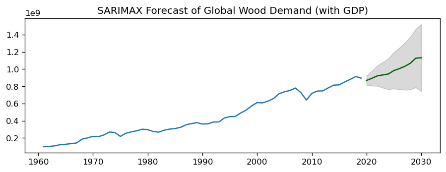
Now that we have created our optimal model, let’s make a prediction about how Global Wood Demand evolves during the next 10 years.

n_periods = 11
fitted, confint = sxmodel.predict(n_periods=n_periods,
                                  exogenous=worldgdp.query("Year>2019")[['WorldGDP']],
                                  return_conf_int=True)

index_of_fc = pd.Series(pd.date_range("2019-01-01", periods=n_periods, freq="Y"))

# make series for plotting purpose
fitted_series = pd.Series(fitted, index=index_of_fc)
lower_series = pd.Series(confint[:, 0], index=index_of_fc)
upper_series = pd.Series(confint[:, 1], index=index_of_fc)

# Plot
plt.plot(data.Value)
plt.plot(-fitted_series, color='darkgreen')
plt.fill_between(lower_series.index, 
                 -lower_series, 
                 -upper_series, 
                 color='k', alpha=.15)

plt.title("SARIMAX Forecast of Global Wood Demand (with GDP)")
plt.show()

And voilá - we have made a prediction about the future in less than one hour, using machine learning and python:

Training Dataset

Of course, we have to critically evaluate our forecasting model, and in the best of the cases compare it to alternative models to be able to identify the best fit. How can we do that? Read my next blogpost, in which I compare several forecasting models and show you, which metrics to use to choose the best one among severals.