Event Studies with heterogeneous treatment effects

Event Studies - Application to dynamic events

In my previous blogpost, I have summarized some research about the flaws of event studies. But can we apply our event study design to settings in which treatments happen at different points in time across units? This is exactly what Sun and Abraham (2020) discuss in their working paper. They show that in these kind of settings, the estimate of a given coefficient can be contaminated by the effect from other periods. Therefore, apparent pre-trends can arise from the sole effect of contamination and treatment effect heterogeneity. They derive an alternative estimator, that is free of this contamination.

They follow Roth (2020) and survey the same 12 papers in top economic journals, but this time focusing on staggered difference-in-difference approaches, reporting, what they call relative period coefficients \(\mu_l\). Sun and Abraham (2020) focus on cohort-specific average treatment effects, the so-called \(CATT_{e,l}\), in which a cohort represents all individuals receiving their first treatment \(E_i\) at the same time \(e\). They then use these \(CATT_{e,l}\) to decompose the relative period coefficients \(\mu_l\). While \(\mu_l\) should only capture the cohort-average treatment effect from period l, the authors find that this is not the case when parallel trend assumptions are violated. Under the parallel trend assumption, we can describe \(\mu_l\) as a linear combination of \(CATT_{e,l}\). The problem with this is that the weights in this linear combination can be non-convex, and even include non-zero weights for relative periods unequal l. These non-zero weights are not what researchers want to show when conducting event studies.

What does this mean for applied work? It means that we can have a spurious non-zero positive lead coefficient even when there is no pretrend. The contamination of \(\mu_l\) from other periods \(l'\) depends on the relative weights on \(CATT_{e,l'}\). These weights, on the other hand, depend on the cohort composition. Examining these weights can give researchers some insight about a potential spurious pre-treatment trend. Sun and Abraham (2020) develop an estimator that can accomodate these heterogeneous treatment effects. Their estimation strategy first estimates the heterogeneous treatment effect of each cohort, and then calculates the average of these cohort-specific estimates through applying cohort-specific weights. They then repeat the analysis with the inclusion of covariates. Importantly, in their specification the \(CATT_{e,l'}\) is the cohort-specific average change in outcome relative to never being treated. This is different to a specification of \(CATT_{e,l'}\) as the cohort-specific average change in outcome relative to being treatment at a different time period (see Athey and Imbens (2018).

Sun and Abraham (2020) show the validity of their estimation method applying it to the research question addressed by Dobkin et al. (2018) about the economic consequences of hospital admissions for adults. The blogpost at hand will summarize their paper in greater detail.

Defining event studies

Sun and Abraham (2020) define event studies as follows. They focus on absorbing treatment, which means that once the treatment status is switched on, it stays on. They estimate the following equation:

\(Y_{it} = Y_{it}^(E_i) = Y{it}^\infty + \sum_{0 \leq e \leq T} (Y_{it}^e - Y_{it}^\infty) \times 1 { E_i = e}\),

where unit i is first treated in time period e. For never treated units \(E_i = \infty\). All individuals for which treatment first switches on in period e form one cohort. It is important to stress that the authors define the treatment effect as the difference between the outcome of treated individuals \(Y_{it}\) relative to the outcome of never treated units \(Y_{it}^\infty\). They then define the \(CATT_{e,l}\) (the cohort-specific average treatment effect on the treated) as the average of all treatment effects of all individuals receiving treatment for the first time at period e. They estimate the CATT not at time period t, but at relative time period l (l periods from the initial treatment e):

\[CATT_{e,l} = E(Y_{i,e+l} - Y_{i,e+l}^\infty | E_i = e)\]

They shift from calendar time t to relative period l as they then can compare across cohorts which received the treatment for the first time at different time periods e, while holding their exposure to the treatment constant.

Identifying assumptions

There are three identifying assumptions in this set-up:

• Assumption 1: Parallel trends in baseline outcomes: This is a generalization of the parallel trend assumption we already know from our canonical DiD Set-Up, and implies that parallel trends should hold for all units receiving treatment for the first time at different periods e, and also for never treated units.

• Assumption 2: No anticipatory behavior in \(l \in g\) periods prior to treatment. This means, that outcomes prior to the treatment should be equal to the baseline outcome, on average. If this assumption holds, then there are no pre-trends, as \(CATT_{e,l} = 0\). This assumption is similar to the no-manipulation of treatment status assumption in the Regression Discontinuity Design. This is most likely to hold if individuals cannot predict their future treatment status.

• Assumption 3: Treatment effect homogeneity: For each relative period l, \(CATT_{e,l}\) does not depend on the timing of its first treatment status e, and is equal to \(CATT_l\). This means that treatment effects are the same across different cohorts for every relative treatment period l. This means that different cohorts share the same treatment path, and does not mean that dynamic treatment effects do not occur. A variation across cohorts could stem from differing covariates across cohorts (e.g. treatment varies by age, and cohorts vary by their age structure), calendar-time varying effects (e.g. macroeconomic conditions), or individuals selecting into treatment at certain times e, that is, the treatment timing is not random. The last case still satisfies their parallel trend assumpion, if it is not determined by the outcome.

Estimators - How to interprete coefficients in the dynamic set-up

The traditional event study regression, also called two-way (unit and time) fixed effects regression, with i=1, …, N units and t=1, …, T calendar time periods looks as follows:

\(Y_{i,t} = \alpha_i + \gamma_t + \sum_{g \in G} \mu_g 1{t-E_i \in g} + \nu_{i,t}\),

where \(Y_{i,t}\) is the outcome of interest for unit i at time t, and \(g \in G\) are relative periods. \(\mu_g\) are the relative period coefficients, and ideally these should be convex averages of \(CATT_{e,l}\). Sun and Abraham (2020) have a closer look at the relative period indicator \(1 {t - E_i \in g}\) to see how it varies with time. They define the following as an indicator for unit i being observed l periods away from the initial treatment at calendar time t:

\[1\{t-E_i \in g\} = 1\{t-E_i = l\} = \sum_{l \in g} D_{i,t}^l\]

This indicator can be applied to a static or dynamic set-up. The static set-up assumes that \(g= [0, T]\) and that \(1{t-E_i \in g} = 1{E_i \leq t}\) (has unit i received its initial treatment by calendar-time period t?). The static regression thus looks as follows:

\(Y_{i,t} = \alpha_i + \gamma_t + \mu_g \sum_{l \geq 0} D_{i,t}^l + \nu_{i,t}\),

The dynamic specification allows for treatment leads and lags, excluding distant ones that are more thanKperiods before treatment and more thanLperiods after treatment, as well as the period before treatment, or period -1. G is \(\{\{-K\},...,\{-2\}, \{0\}, \{1\},...,\{L\}\}\), and the dynamic regression looks like:

\[Y_{i,t} = \alpha_i + \gamma_t + \sum_{l = -K}^-2 \mu_l D_{i,t}^l + \sum_{l = 0}^L \mu_l D_{i,t}^l + \nu_{i,t}\]

The exclusion of some relative period is necessary to avoid multicollinearity. Excluding the period prior to to treatment is common practice. Another common practice is to bin or trim distant periods.

Sun and Abraham (2020) next inspect the relative period coefficients under a combination of the assumptions listed above:

• They show that under no assumptions the coefficient \(\mu_l\) is a linear combination of differences in trends from its own relative period \(l \in g\), from other relative periods \(l \in g'\), and from excluded relative periods, weighted by weights \(\omega_{e,l}^g\). They show that for \(\mu_g\)’s own relative period, the weights sum up to 1, for other relative periods, the weights sum up to 0, and for for excluded relative periods, the weights sum up to -1. For never treated units, the weights are zero.

• Under the parallel trend assumption only, \(CATT_{i,l}\) is a linear combination of the CATT belonging to its own relative period, and other relative periods. The weights in this case can be non-convex, and it is important to examine them, to see if one particular CATT is driving the overall estimate (treatment heterogeneity does matter).

• Under the parallel trend assumption, and no anticipation assumtpion, \(CATT_{i,l}\) is a linear combination of post-treatment \(CATT_{e, l'}\). What does this mean for applied work? This means that pre-trend tests based on pre-period coefficients are invalid, if effects are homogeneous across cohorts. Non-zero pre-treatment coefficients do not automatically give evidence of pre-treatment trends. This is due to the fact that under the no-anticipation assumption the coefficients of all cohort-specific treatment effects prior to treatment are all zero, and therefore also their linear combination. But still, due to the influence of post-treatment \(CATT_{e \geq 0}\) the estimant is not necessarily zero. Therefore, traditional pre-trend tests are invalid.

• Under the parallel trend assumption, the no-anticipation assumption, as well as the treatment effect homogeneity assumption, \(CATT_{e,l} = CATT_{l}\) is constant across e for a given l and \(\mu_g\) is equal to a linear combination of its own relative period CATT minus the linear combination of the CATT from other relative periods.

Alternative estimation method - the interaction-weighted estimator

Sun and Abraham (2020) propose a new estimation method that is robust to treatment effect heterogeneity, and generate an interpretable relative period estimator \(\mu_g\) with non-negative weights that sum up to one. They create the following weighted-average, with weights being the share of cohorts that experience their first treatment in period e, or at least l periods relative to the treatment, normalized by the size of g:

\[\nu_{g} = \frac{1}{|g|} \sum_{l \in g} \sum_e CATT_{e,l} Pr \{ E_i = e | E_i \in (-l, T-l) \}\]

To estimate \(\nu_{g}\) the authors first estimate each \(CATT_{e,l}\) and then estimate their respective weight using their sample analogs. They then average across the respective cohort-specific estimates. They call their estimator an interaction-weighted estimator. The exact procedure is as follows:

• Step 1: Estimate the \(CATT_{e,l}\) through a linear two-way fixed effects specification that interactsrelative period indicators with cohort indicators

• Step 2: Estimate the weights by sample shares of each cohortin the relevant period(s)

• Step 3: Estimate a weighted average using Step 1 and Step 2 to generate the IW-estimator

Bringing it to practice - Some empirical illustrations

Sun and Abraham (2020) illustrate their results applying it to the work conducted by Dobkin et al. (2018). Dobkin et al. (2018) examine the economic consequences of hospital admissions for adults, applying an event-study and to two different datasets: The Health and Retirement Study, as well as hospitalization data linked to credit reports. They use 20 years of the Health and Retirement Study (1992 - 2012) to analyze the impact of hospital admissions on out-of-pocket medical spending, income, and its components, focusing on 2,700 insured adults between 50-59 years old. Second, they analyze a 10-year panel (2002-2011) of merged credit reports and hospizalization data, focusing on 380,000 adults with health insurance between 25-64 years old. They find “sharp, on-impact effects of hospitalizations that in many cases persist, or even increase, over time”.

Dobkin et al. (2018) estimate a parametric and non-parametric event study. The non-parametric event study estimates the effect of the treatment of interest for relative time (time relative to the event), allowing for a flexible estimation of treatment patterns relative to the event time:

\(y_{it} = \gamma_t + X_{it} \alpha + \sum_{r=S}^-2 \mu_r + \sum_{r=0}^F \mu_r + \epsilon_{it}\),

with \(\gamma_t\) being calendar-time fixed effects, \(X_{it}\) being covariates, and \(\mu_r\) being the coefficient on indicators for time relative to the treatment, here hospital admission. The omitted category is \(\mu_{-1}\), and the estimator of interest are the relative treatment effects to this omitted category.

In the HRS data, event time r is the survey wave relative to the survey wave during which the event is reported to have ocurred (r = 0). The author analyze three waves prior to index admission (S=-3), and three waves after index admission (F=3). As the HRS data is biannual, the authors include biannual survey wave indicators that control for calendar time (\(\gamma_t\)), and include “HRS-cohort”-by-wave dummies (X_it) due to sample composition changes. For the credit data, which is gathered once per year in January, the relative time dimension is months, as individuals are admitted to the hospital during different months within the year. They limit the sample to relative months from -42 to 72. The omitted category (\(\mu_r\)) is the month prior to hospitalization. \(\gamma_t\) are calendar year-fixed effects. The underlying identification assumption is that the timing of hospital admission is unrelated to the outcome of interest. This assumption would be violated if individuals are admitted to hospitals due to job losses, or if they were an a downward health-trend prior to hospital admission, and anticipated the hospital admission. The non-parametric event study allows for an examination of these possible threats, and consequently, serves as the basis for the functional form assumptions of the parametric event study:

\(y_{it} = \gamma_t + X_{it} \alpha + \delta r + \sum_{r=0}^3 \mu_r + \epsilon_{it}\),

which allows for a linear pre-trend in event time r. The coefficient of interest \(\mu_r S\) then shows the change in outcome following a hospital admission, relative to any preexisting linear trends. The credit report specification further includes cubic spline in post-admission event time, allowing for second and third derivatives of the relationship between outcome and event time to change after r>0, the fourth derivative after r>12, and the fifth derivative after r>24. The functional form specifications for both datasets are based on the nonparametric event study, and the figures below:

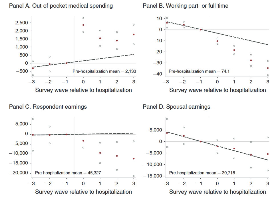
The authors observe some heterogeneity across treatment effects for different age groups as well as socioeconomic groups. They test their findings to alternative specifications to assess robustness. These are the inclusion of individual-fixed effects, a balanced panel, wave fixed effects only, adding demographic covariates, a non-restriction of pre-period observations, as well as a poisson distribution.

Sun and Abraham (2020) state the paper by Dobkin et al. (2018) suits their purpose, as the parallel trend assumption as well as no anticipation assumption are likely to hold, but there seems to be heterogeneity across cohorts due to cohort compositional changes. They estimate an event-study regression estimation with three leads and lags, including an indicator variable for each lead and lag (see equation 22 in their paper). In contrast to the original paper, Sun and Abraham (2020) do not trim the sample, but balance it over calendar time. They then exclude the period before hospitalization (l=-1) and l=-4. They then focus on the coefficient \(\mu_0\) that supposedly captures the contenmporaneous effect of hospitalization. They show that \(\mu_0\) is a linear combination of the CATTs from its own relative period, as well as other relative periods, and the excluded periods. They plot the waves of each of the CATTs:

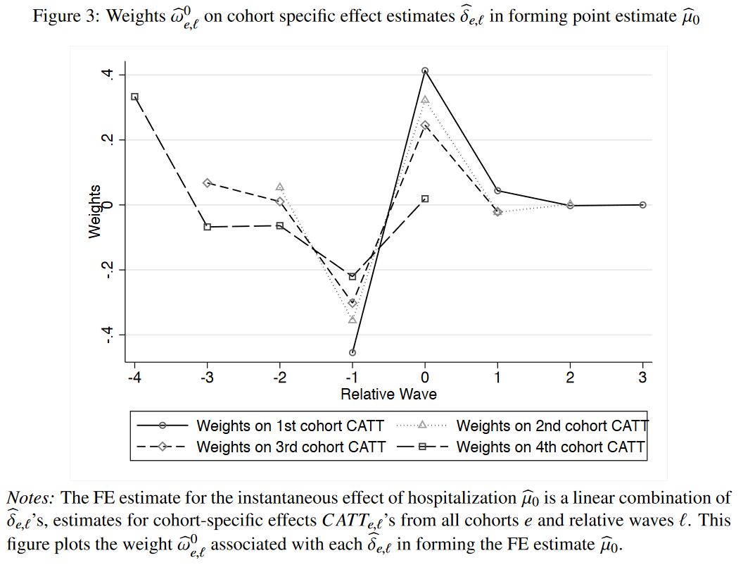
The figure above shows that weights are large for leads of treatments (negative relative waves), and therefore our contemporaneous estimator \(\mu_o\) is sensitive to pre-trends. Consequently, it does not isolate the contemporaneous effect of hospitalizations. Therefore, in a next step, Sun and Abraham (2020) estimate their IW estimator, and show, that the estimators are very similar to the traditional FE estimators. Still, the two-way fixed effects estimators are marked by non-convex and non-positive weights.