
Event Studies and their flaws
Event Studies - Giving them a critical close-up
As already mentioned in my previous blog post about what event studies are a recent paper by Roth (2020) gives event studies a critical close-up, especially about the fact that they are often used to test parallel trend assumptions. Analyzing 12 papers applying event studies in leading journals, he finds that tests are often underpowered, and that distortions from pre-trends is a concern. He also introduces some methods that improve upon the standard testing of pretests.
Giving an example, in which linear pre-trends exists, he shows that even in this case, sometimes these linear trends are rejected. The failure to detect these linear trends then leads to a bias that is worse then under the scenario, in which we acknowledge them. This is due to the fact that the linear pre-trends are masked by noise in the data, and that this noise then also worsens the bias in respective treatment-effect due to mean-reversion. In general, the bias from these masked pre-trends can be smaller or larger than the traditional bias due to acknowledged pre-trends, but in the case of homoskedastic standard error and a monotonic difference in trends the bias is always large than the unconventional one. The masking of linear pre-trends also affects the variance. Roth (2020) shows that the variance of conventional estimates is lower conditional on passing the pre-test.
Roth (2020) presents several possible solutions to this problem. Of course, all of these proposals are based on assumptions about the violation of parallel trends themselves. Therefore, we have to decide on a certain method, depending on which assumption we believe to be true in our respective case. The proposals presented by the author are:
-
The extrapolation of the pre-treatment difference in trends to the post-treatment periods via a functional form assumption. The problem with this approach is that researchers are often unsure about the correct functional formfor the differential trend. Therefore, he proposes an alternative approach that relaxes the exact parallel trends assumption:
-
Freyaldenhoven et al. (2019) allow for a violation of the parallel-trend assumption as long as there exists a covariate that is unaffected by the treatment, but by the same confounding factor leading to pre-trend differences.
-
Rambach and Roth (2019) propose to conduct a form of sensitiviy analysis to the parallel trend assumption, and through this find out how and when it affects the estimated treatment effect.
Roth (2020) introduces a model with three periods, homoskedastic errors, and (potentially) linear violations of parallel trends. This means that we have an outcome \(y_{it}\) for individual i that we observe in the three time periods t=-1,0,1. The individuals can forme part of the treatment group (\(D_i = 1\)), or the control group (\(D_i = 0\)). We then have two potential outcomes \(y_{it}(1)\) and \(y_{it}(0)\). Now let’s assume that there is no causal effect of the treatment and \(y_{it}(1)\) = \(y_{it}(0)\), and that:
\(y_{it}(0) = \alpha_i + \theta_t + D_i \times g(t) +\epsilon_{it}\),
where \(D_i \times g(t)\) is a potential difference in trends between the treatment and control group. With \(g(t)=t\) the outcome of our treatment group is linearly increasing relative to the outcome of our control group, but if \(g(t)=0\) then our parallel trend assumption holds, and there are no pre-treatment trends present.
Roth (2020) then applies a traditional Difference-in-Difference specification, that is:
\(y_{it}= \alpha_i + \theta_t + \sum_{s \neq 0} beta_s × 1[s=t] \times D_i + \epsilon_{it}\).
\(\beta_1\) is our canonical difference-in-difference treatment effect, and \(\beta_{-1}\) our pre-period event-study coefficient. Importantly, \(\triangle y_{t=0}\) enters the formular for both estimates (the post- and pre-coefficient). This is important, as if we assume \(\beta_{-1}\) to be 0, this affects our distribution of \(\triangle y_{t=0}\), and this on the other hand influences the distribution of \(\beta_{1}\). This is important to have in mind for the argument Roth (2020) is making.
In his paper, he assumes a linear violation of the parallel trend assumption \(g(t) = \gamma \times t\), and that \(Var[\beta_1] = Var[\beta_{-1}]\). He then examines the characteristics of the point estimate under the survival of the parallel trend assumption. The left panel of the figure below shows the probability of passing the pre-test of not having a significant coefficient \(\beta_{-1}\) at the 95%-level. This means, that we fail to find a significant effect of pre-trends in 95% of the cases (\(\gamma\) on is equal to 0). Still, let’s have a closer look at the graph, for example for values of \(\gamma = 2\) (equivalent to the mean of \(\beta_{-1}\) being two standard errors below 0, and the value of \(\beta_{-1}\) being between 0 and 4 on our x-axis of the graph). The graph shows us that we then reject the pre-test with a probability of 0.5. In 50 percent of all cases, we pass the pre-test of \(\beta_{-1}\) being zero, although it clearly is not zero!
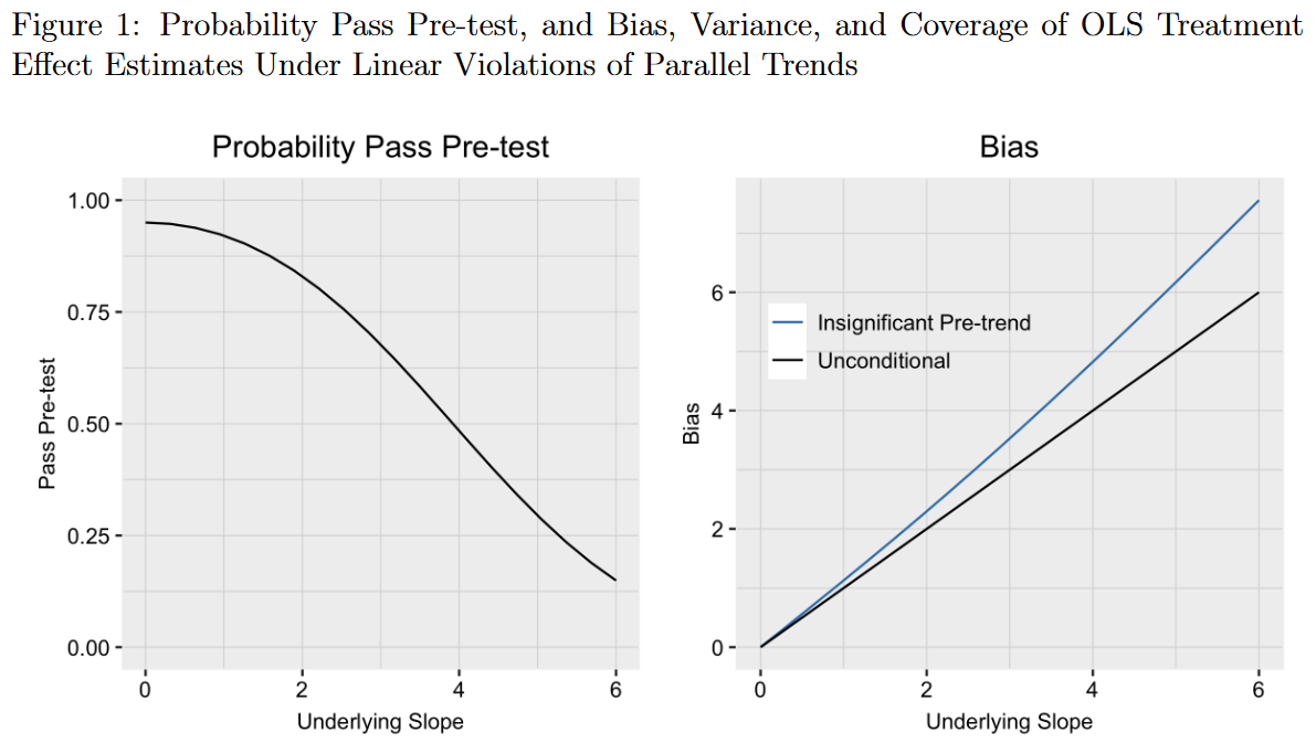
The right panel of the figure above shows the bias of our estimate. Roth (2020) shows that in the case without conditioning on parallel pre-trends the bias simply is equal to the underlying true difference in trends \(\gamma\) (the black line). But if we condition on parallel trends, but did not detect the actual underlying difference in trends, our bias is larger than in the unconditional case (the blue line). But where does this increased bias come from? The figure below explains this in more detail. The left panel plots \(\triangle y_{t}\) (the difference in sample means between the treated and control group in period t) for hte case where \(\gamma = 3\). The observations in blue are draws from the data where no pre-trend difference is observed, having smaller slopes in the pre-treatment period post-treatment period (by construction). The same observations have a steeper slope in the post-treatment period, representing an increased bias in our post-treatment period. Where does this come from? Roth (2020) explains that this is due to \(\triangle y_{t=0}\) having below-average values. This is due to negative shocks in period 0, and a flattening of the observed slope in the pre-treatment period. The mean-reversion process than leads to increased slopes in the post-treatment period, resulting in biased estimates for period 1.
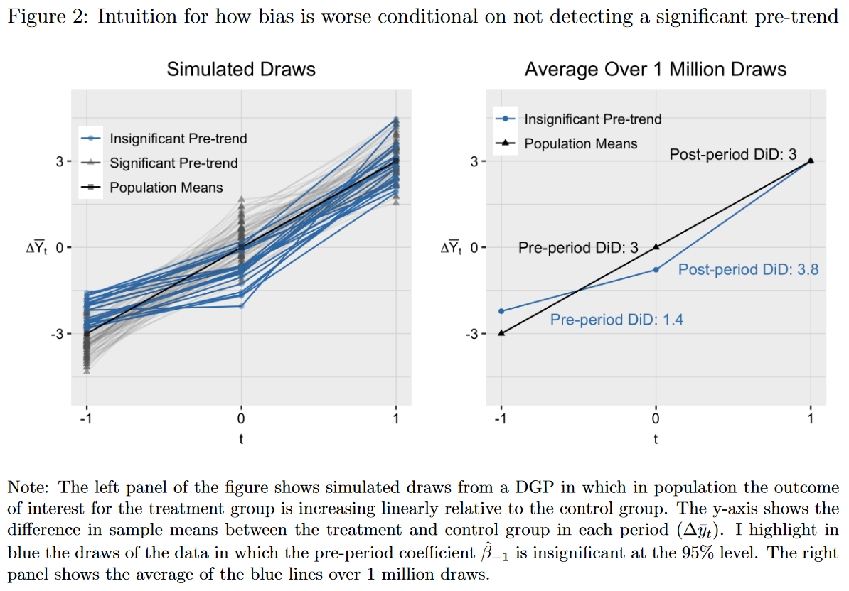
Roth (2020) also shows that the false non-rejection of parallel trends affects our variance estimator. The variance of passing the pre-trend test is lower than the unconditional variance. This can also be seen in the figure above. The blue dots are less disperse than the grey triangles. The combination of this variance effect, and the bias effect described in the paragraph above then leads us to conventional CIs that over-cover for pre-treatment differences in trends close to zero, and under-cover in the case of large pre-treatment differences.
In his paper, Roth (2020) also develops the general model of the three period case discussed above, but in the virtue of time I will refer you to his paper for that. I will focus on the implications he derives for applied work. Reviewing a number of papers in leading journals he shows that conventional pre-tests for parallel trends often have low power even against substantial linear violations of parallel trends. As mentioned above, he then presents alternative methods to apply if we suspect our parallel trend assumption to be violated.
The first possibility is to impose particular functional form restrictionson the way that parallel trends can be violated. We can then extrapolate pre-treatment data to our post-treatment periods, and estimate the counterfactual difference in trends, and removing the bias in conventional estimates. One possiblity there is to assume linearity in the violation of pre-trends, that is \(\delta_t = t \times M_t \delta_{pre}\). We then have \(\tau_t = \beta_t - t \times M_T \beta_{pre}\), a valid causal estimator, under the assumption that the functional form specification is correct. The downside of this solution is that often it is not possible to identify the correct underlying functional form, and that the exact functional form remains an open question.
Therefore, Roth (2020) refers to alternative solutions to relax the parallel trend assumption without relying on these strong assumptions about the underlying functional form of the parallel trend violation. One such approach is the one proposed by Freyaldenhoven et al. (2019). They allow for a differential trend in the outcome \(y_{it}\) as long as this difference is driven by an unobservable variable \(\eta_{it}\) that also affects treatment status \(D_{it}\), and as long as we observe an alternative outcome \(x_{it}\) that is also affected by \(\eta_{it}\), but unaffected by treatment \(D_{it}\). This line of thinking is similar to what we know from instrumental variable approaches. the downside of this approach though is that it is often difficult to find the excluded outcome variable \(x_{it}\).
Rambach and Roth (2019)’s approach is based on the assumption that the difference in pre-trends is based on some pre-specified class \(\triangle\), and imposes smoothness restrictions. The authors recommend to conduct sensitivity analysis with respect to the linearlity assumption in differential trends. Through these sensitivity analyses researchers can then deduce conditions under which certain conclusions hold.
The paper by Roth (2020) stresses an important point relevant for research applying event-studies, or difference in difference. It is not enough to simply rely on a non-rejection of parallel trend assumptions. Researchers should think about what the parallel trend assumption actually implies from an economic viewpoint, and then deduct reasonable assumptions about the functional form of this assumptions. The methods presented can then serve to stress the robustness of causal inferences made.
For flaws in Event Studies with varying treatment, see the paper by Sun and Abraham (2020) which I resume in my next blogpost.