
Event Studies - What do they show, and why do we need them?
Event Studies: What is an event study?
Often in economic papers that use Difference-in-Difference, or the staggered version of it, we can observe that researchers conduct event studies as robustness tests. A recent working paper by Jonathan Roth (2020) reflects on this method, and the fact that economists often apply event-studies to test for pre-trends (or the famous parallel trend assumption). He finds that over 70 journals published in the AEA report an event-plot. He then shows that the power of these tests is often low, and that distortions from pre-testing is a concern.
But before getting on the details on this, let’s revise what it actually means to conduct an event study. Therefore, let’s have a look at the paper by Lafortune et al.(2018). They study the impact of post-1990 school finance reforms on student achievement in low-income school districts, using an event-study design and nationally representative data. The authors show that educational spending as measured by real per pupil revenues has constantly increased between 1990 and 2012. They argue that most of these increases are due to school finance reforms, directed at low-income districts.
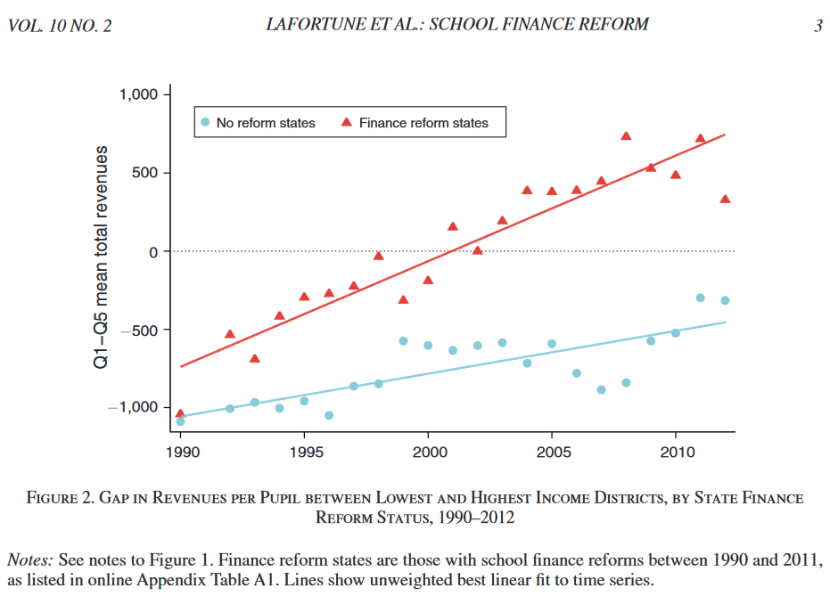
They construct a state-by-year panel based on fourth- and eighth-graders taking a yearly math and and reading test. They employ an event study to distinguish the effects of the reforms from other potential determinants of these test-score cards. The event study suits their purpose as the reforms were implemented randomly across states and time. They state that there are 64 school-financed reform events in 26 states between 1990 and 2011. Of these 26 states, 18 had multiple events. The states that do introduce a reform in a certain year forms the treatment group in this set-up, while states without a reform form the control group, after accounting for fixed effects at the state and year level. Following this, the estimation equation looks like that:
\[\theta_{st} = \delta_s + \kappa_t + 1(t>t_s*) \beta_{jump} + \epsilon_{st}\]Here, \(\theta_{st}\) is the outcome of interest in state s and year t, \(\delta_s\) is the state-fixed effect and \(\kappa_t\) is the year-fixed effect. \(\beta_{jump}\) is our main coefficient of interest, with \(t_s*\) representing the time of the event in state s. As the event is assumed to be permanent, the equation considers t>\(t_s*\). Standard errors are clustered at the state level. As indicated above, the identifying assumption of this equation is that events (reform) were rolled-out randomly, and that without the reform taking place, outcomes (spending and student achievement) would have developed parallely in treated and untreated states. The authors state that this assumption might be too ambitious, and therefore decide to focus on relative student outcomes, instead of absolute student outcomes. What does relative in this case mean? They simply compare outcomes of high- and low-income districts in the same state. With this outcome, different underlying trends or confounders across states and years do not affect our parallel trend assumption anymore, as long as they affect low- and high-income districts within the same state similarly. The identification assumption under this specification changes to that relative outcomes of low-income districts would have followed parallel trends across states in the absence of SFRs. This is what we call a triple difference strategy.
The unit of observation in their paper are districts. Therefore, the authors aggreggate the student achievement data by district, and then merge it to additional district-level data. The student achievement outcomes is then on the district-year-grade-subject level, pooling data from 1990 to 2011. For the student achievement outcome they then also use year-grade-subject fixed effects, instead of simple year fixed effects.
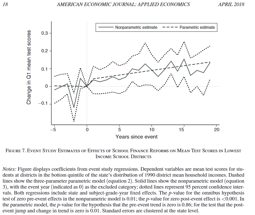
Lafortune et al.(2018) test for parallel trends before the implementation of the reforms and find that there are no systematic changes in the periods leading up to the reform. They find clear changes in student achievement after the reforms. Ten years after a reform, relative achievement of students in low-income districts has risen by roughly 0.1 standard deviation.
Event Studies: What if events are not random, or take some time to be fully implemented?
There are two possible threats to the estimation equation shown above. First of all, SFRs may materialize gradually, especially when talking about student achievement outcomes. As a student’s achievement not only depends on the quality of education that s/he receives after the reform, but also before, the development of results may be gradual. Another threat to the identification stratey would be the violation of our assumption that events occur randomly. If states experiencing events systematically differ from events not experiencing events, then this might lead to a bias. Lafortune et al.(2018) solve this by adding two trend terms:
\[\theta_{st} = \delta_s + \kappa_t + 1(t>t_s*) \beta_{jump} + 1(t>t_s*)(t-t_s) \beta_{phasein} + (t-t_s) \beta_{trend} + \epsilon_{st}\]\(\beta_{phasein}\) represents delayed event effects, capturing annual changes in the outcome in state s after \(t_s*\) and relative to t, while \(\beta_{trend}\) represents a falsification test. If \(\beta_{trend}\) is unequal to 0, this would mean that our randomization assumption does not hold.
Lafortune et al.(2018) additionally estimate a non-parametric version of the estimation equation to allow for non-linear phase-out effects of the treatment, as well as non-linear pre-trends:
\[\theta_{st} = \delta_s + \kappa_t + \sum_{r=kmin}^r=kmax 1(t=t_s* + r) \beta_{r} + \epsilon_{st}\]In the equation above \(\beta_{r}\) can be interpreted as the effect of an event taking place in year \(t_s*\) r years later, relative to r=0, and with r being censored at kmin=5 and kmax. This specification then shows that the treatment effect is sometimes spread out over a view year following the event. The authors only reject the non-significance of pre-event coefficients once, as shown in the figure below.
Summing up: How to use event studies in economics
The paper presented in this blogpost shows how to use an event study as your main identification strategy. But often, papers employ a Difference-in-Difference strategy and then employ event studies to shed some light on the dynamics behind treatment effects, and to show that the parallel trend assumption is fulfilled. One example is the paper that I discussed in one of my previous blogposts about Staggered Difference-in-Difference. Hoynes et al. (2016) conduct an event study to raise insights about the question on when investments in children actually most matter. This also helps to further interpret the magnitude of the treatment effect, and the underlying parallel trend assumption of their estimation. Contrary to the estimation equation of their Staggered Difference-in-Difference Design, they recode their main effect \(FSP_{cb}\) to a series of dummies that is one for two-year intervals of the age at FSP introduction. They omit the 10-11 age category and trimm age at 12 and 5 years respectively to reduce collinearity between event tme and birth year.
Their event study confirmed their hypothesis of larger treatment effects for children who are exposed to the FSP earlier and therefore for a longer time period.
And are there any shortcomings with these event studies?
Indeed, there are. As already mentioned in the beginning, there are flaws to these event studies, especially when using them to test for parallel trends. Jonathan Roth (2020) gives this a critical look, and so do Athey and Imbens (2020). I will discuss their insights in my next blogpost.