
Staggered Difference-in-Difference - What is different?
Staggered Difference-in-Difference: What does it mean?
Often, a policy is introduced in many different states during many different time periods. This is what researchers refer to when they talk about a staggered Difference-in-Difference Design, or a generalized Difference-in-Difference. Let’s have a look at the food stamp program. The food stamp program was rolled out on a county-by-county basis between 1962 and 1975. The program provided low-income families with food vouchers that could be used at grocery stores. A paper by Hoynes et al. (2016) uses this staggered roll-out as their identification strategy to assess the long-run effects of childhood access to the safety net. They analyze the participation in the program, and with this, an increase in income and resources, on health and economic outcomes in the long-run. Their main treatment variable is the time period that children were subject to the program between conception and the age of 5. The graph below from their online appendix shows the staggered implementation of the Food Stamp Program (FSP) over time (Note: The numbers in the figure is weighted by the 1970 county population):
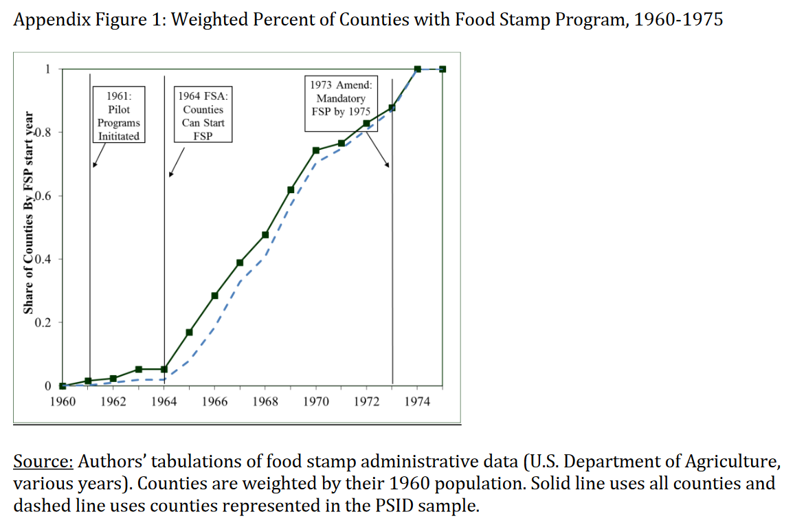
The image shows that the FSP started with a pilot program in 1961, a pilot expansion phase from 1962 to 1963 to 43 counties, and the Food Stamp Act of 1964, giving all states access to the program, leading to a steady stream of counties implementing the FSP from 1964 onward. The FSP became mandatory in 1975. The authors use this variation as their identification strategy, with the month of FSP adoption representing the start of the treatment. Taking the difference between the month and year of the respective FSP introduction in a specific county and birhtmonth and birthyear of children born in this specific county, the authors construct their main explanatory variable and their measure of childhood exposure to the FSP.
Their sample consists of children born between 1956 and 1981. This sample contains several pre- and post-treatment cohorts, as well as children born along the full rollout period of the FSP. Their data comes from the PSID data from interview year 2009. Therefore, the oldest individual in their sample is 53 years old. They limit the sample to people who are older than 18 years old for their health outcome (through introducing a dummy), and older than 25 years old for the economic outcome (through introducing another dummy). The authors also introduce the following control variables: Family background variables during early life, county-level controls from 1960, and county-year controls (number os hospital beds, hospitals per capita, real (non-FSP) government tranfers per capita, and a dummy for having a community health center).
They estimate the following equation: \(y_{ibc} + \alpha + \delta FSP_{cb} + X_{icb}\beta + \eta_c + \lambda_b + \gamma_t + \theta_s \times \beta + \phi CB60_c \times \beta + \epsilon_{icb}\),
with i indexing the individuals, c indexing the county of birth, b indexing the birth year, s indexing state of birth, and t the survey year. The main variable of interest is FSP, the measure for food stamp availability in early life. The authors measure its exposure by the share of months that the food stamps were available in the adult’s birth county. As counties adopted the FSP at different points in time, I have variation across birth counties as well as birth cohorts. This is the famous traditional Difference-in-Difference estimation, that I talked about in my previous blogpost. One difference stems from differences across counties within the same birth cohort, while the other difference stems from differences within counties across different birth cohorts (those born later are more exposed to the program than those born later). Importantly, the estimation above estimated the intent-to-treat-effect, that is the intention to treat the whole underlying population. This is different from the average treatment effect, as not all individuals the program intents to address actually participate in the program (the pick-up of the program is not 100%).
As you can see in the equation above, Hoynes et al. (2016) introduce a variety of fixed-effects in their equation: Unrestricted cohort effects at the national level (\(\lambda_b\)), unrestricted county effects (\(\eta_c\)), unrestricted interview year effects (\(\gamma_t\)), as well as state-specific linear year of birth trends (\(\theta_s \times \beta\)). They also control for a set of individual-level controls (\(X_{icb}\)), as well as trends in the observable determinants of FSP adoption (\(CB60_c \times \beta\)). Do you wonder why they include pre-treatment county characteristics, interacted with linear time trends? More about this last point in the next paragraph!
Staggered Difference-in-Difference: When does it work?
Exogeneity of treatment adoption
Similarly to the traditional Difference-in-Difference strategy with one period and one treatment and control group, the staggered DiD relies on important assumptions. The most important assumption is the exogeneity assumption. The identification strategy holds, if the rollout is exogenous, that is randomly implemented over time, and not related to variables important for our outcome of interest, or related to the outcome of interest itself. If, for example, the FSP in its early phase was only implemented in areas with low health conditions, and later in areas with high health conditions, our treatment and control groups systematically differ from each other. Or if it first was implemented in areas with a high poverty share, and then in areas with a low poverty share. These differences in county characteristics that influence the adoption timing could result in spurious correlation, if these same county characteristics are related to differential trends in our outcome of interest. The identification assumption is that there are no contemporaneous county level trends that are correlated with the introduction of the FSP and our outcomes of interest at the same time (health and economic outcomes).
How do we test this assumption? First, we can run a regression, in which the adoption of our FSP is the outcome variable, and all kind of pre-treatment covariates are introduced as potential explanatory variables. Hoynes and Schanzenbach (2009) run this regression and find that counties with earlier adoption of FSP are more populous, urban, black, low income and with a smaller fraction of land used in agriculture. The figures below show example graphs for the share of black people, as well as log population.
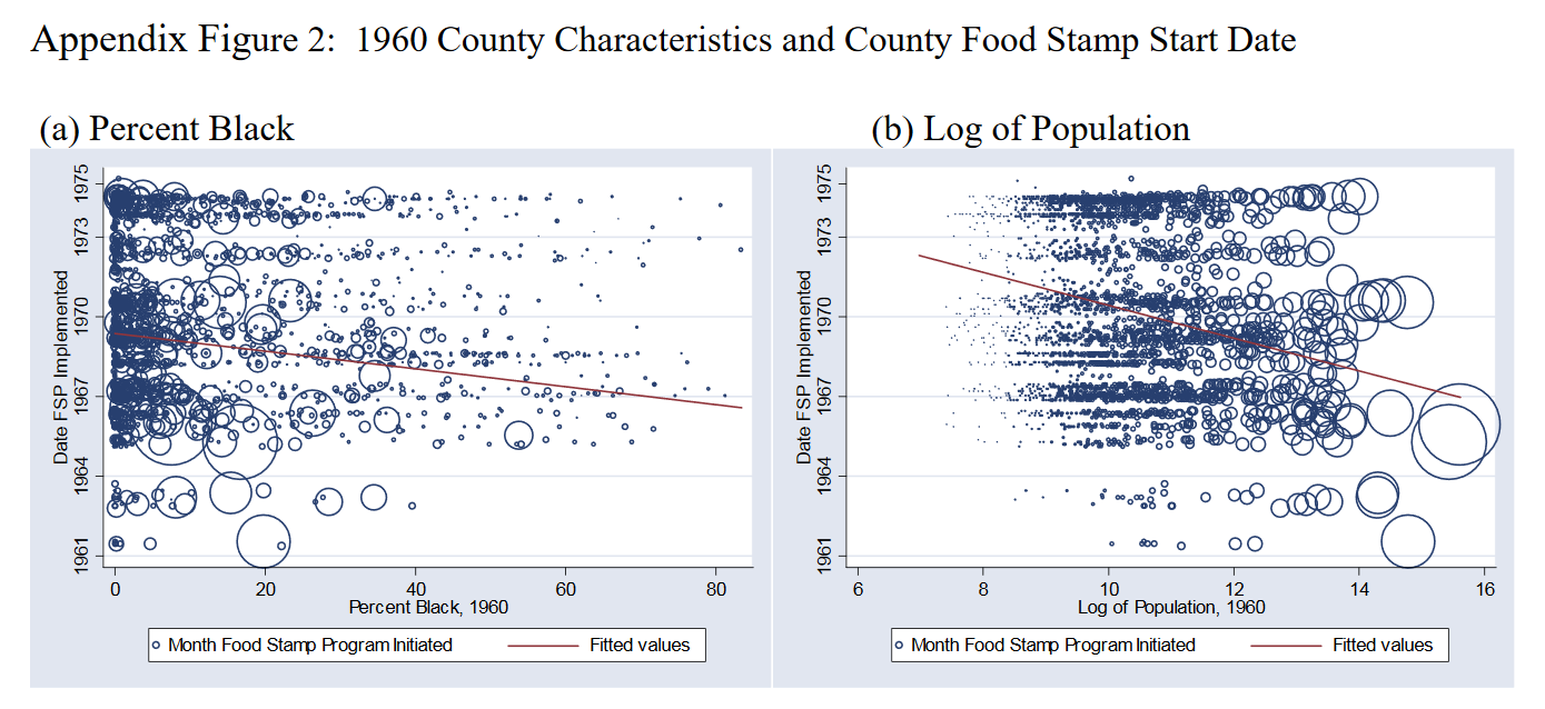
The authors argue that this is not problematic to their identification strategy, as they indeed are significant determinants, but explain very little of the actual food stamp adoption. As the figures above show, the magnitude of the estimate is low and varation high. Still, to control for these possible confounders, they include linear trends interacted with these pre-treatment significant determinants in their estimation equation. This controls for observable, parametric trends across countries, but does not take into account unobservable, non-parametric trends. In their paper they present results for estiamtes with and without state fixed effects, with and without pilot counties. For a detailed overview of their results refer to Table 1 in their AEJ paper.
No confounding alternative programs or policies
Hoynes and Schanzenbach (2009) state that the FSP was introduced during a time of great expansion of programs for the Poor in the US. To take this into consideration, and control for possible confounding programs introduced at the same time, they control for county-by-year controls for federal spending on other social programs. They show that the introduction of this covariate does not significantly change their outcome of interest, confirming the “cleaniness” of their identification strategy.
Staggered Difference-in-Difference: Can we trust it?
In economic papers, you often have to show that your results are robust. What does that mean? You want to show that your results indeed hold, and are not just a result of specific characteristics of how you defined your estimation equation, or your data. Hoynes et al. (2016) conduct some of the most common robustness tests. These are:
- Reestimating the estimation equation for subgroups of the underyling sample
- Adding additional controls, or introducing more fixed-effects
- Conducting placebo tests
- Conducting a triple difference design
- Estimating an event study
In their paper the authors reestimate the equation by gender, to see if either male or female individuals drive the results. They reestimate their results including controls for county programs and resources available between age zero and five, to control for potential confounders. And they conduct a placebo test through restricting the sample to individuals likely to be unaffected by the program (in their case restricting the sample to families with high education). To better understand the Triple-Difference estimation see my latest blogpost on Triple-Difference - Why Triple?. Hoynes et al. (2016) apply a Triple-Difference strategy interacting their treatment variable \(FSP_{cb}\) with the probability of being affected by the program, the group-level food stamp participation rate \(P_g\). The main identification assumption here then is that there are no differential trends for high participation versus low participation groups within early versus late implementing countries.
As many papers applying Difference-in-Difference, and especially staggered Difference-in-Difference strategies, the authors also use an event-study design to confirm the robustness of their results. I will treat this design that slightly differs from the DiD that we have seen so far in this blogpost on event studies.
Also, have in mind that there is an entire new literature emerging that analyzes what the generalized DiD estimate actually is about, and until which degree we can apply traditional interpretations of DiD estimates to a staggered Difference-in-Difference design. I will discuss this literature in a future blogpost.