
Revisiting Difference-in-Difference - Taking the DiD Design to a next level ?
Traditional Difference-in-Difference: What do we need it for?
Often we do not have the money nor the time to conduct field experiments, especially in development countries. Therefore, economists often employ quasi-experimental strategies, taking advantage of so-called natural experiments. Image that you want to exploit the effect of deforestation on poverty. Instead of implementing a field experiment, in which you deforest randomply-selected treatment areas, and leave randomly-selected control areas untouched, you can search for natural experiments. Image that there has been a fire due to lack of rain and heat in a certain region, similar to what has happened in Australia, or also several parts in Latin America. You can simply take this event as a natural experiment, and a sort of “proxy” for deforestation. You can then compare the evolution of poverty over time in the by the disaster affected region to a region that has been unaffected by the event.
This is what economists traditionally call a difference-in-difference design. It is a method that tries to solve the issue of missing counterfactuals. The problem with experiments in general is, that you observe each individual only once. If you try to find out the effect of a certain vaccine, you only observe person i with our without the vaccine. You do not observe this same individual in both states, that is, with and without the vaccine. Therefore, if this person i gets sick after receiving the vaccine, you cannot know if this person would have gotten sick anyways, even without participating in the experiment, or if s/he got sick due to that.
In field experiments you try to solve this issue through two actions: Firstly, you choose a large enough sample to make sure that by coincidence you do not only have people with unknown, underlying health issues in your treatment group, that will all react strongly and badly to the vaccine, while only having super healthy people in your control group, or vice versa. Secondly, you randomly distribute your sample to treatment and control groups, to avoid that treatment and control groups differ on certain observable and unobservable characteristics. If you combine both actions, chances are large that you will get a sample that is representative for your underlying populatoin, leading you to a pretty reliable result of your vaccine’s effect.
Natural experiments try to mimique these field experiments. Let’s have a closer look at the traditional difference-in-difference design, and let’s go back to our wildfire example to better understand it. Analyzing poverty data over time in the region affected by the wildfires won’t do the job to get a full picture, about what is happening. Why? Because we are missing a counterfactual. We are only observing the poverty evolution of people who have been affected by the wildfire. If we know observe that poverty increased for them, it is impossible for us to disentangle this effect from underlying poverty dynamics that would have developed in any case. Maybe the wildfires just arose in this region as its inhabitants were becoming poorer and poorer anyways, and therefore did invest less in protective gear. We cannot observe this, if we don’t have a comparison group.
Difference-in-Difference provides us with a solution for this problematic. What we do in Difference-in-Difference is to take a region that is similar to the region unaffected by the treatment we are interest in, in this case wildfires, and compare the evolution of poverty in our wildfire region (the treatment group) to the evolution of poverty in our control region (the control group). We can then subtract the difference in poverty over time observed in both regions from each other, and have an estimate that is a relatively good proxy for what we are actually looking for.
| Before Treatment | After Treatment | Differences | |
|---|---|---|---|
| Treatment Group | A | B | B-A |
| Control Group | C | D | D-C |
| Differences | A-C | B-D | (B-A) - (D-C) |
The differences across time (B-A and D-C) control for time trends, while the second difference, group differences within time periods, control for selection bias (A-B and C-D). The difference-in-difference design cancels these effects out and leaves us with a credible estimation result.
Traditional Difference-in-Difference: When does it actually work, and what do we need to keep in mind?
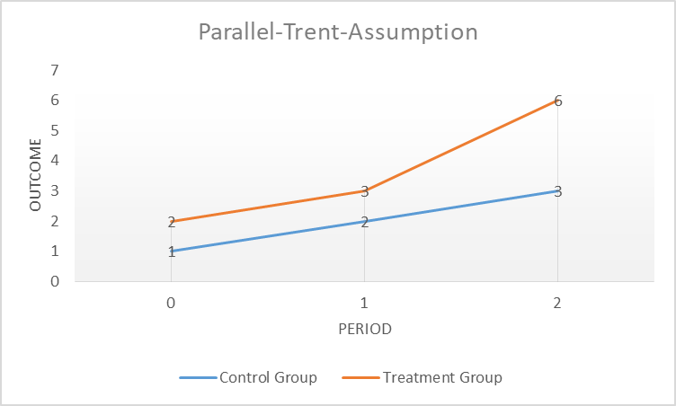
This research strategy only works under an important condition, known under the name “parallel trend” assumption. As discussed previously, it is important for our estimation effect that our treatment and control groups are similar to each other, and therefore comparable, that is, our control group is a good counterfactual for our treatment group. I can test this assumption graphically by plotting our outcome of interest over time and test if they evolve similarly to each other before the imposition of the treatment of interest, in our case, wildfires. The parallel trend assumption therefore controls for the development over time of all observable and unobservable covariates (control variables) that evolve similarly in our treatment and control area. It does not account for covariates that evolve differently between the treatment and control area over time. Let’s assume, for example, that urban infrastructure changes in our wildfire area over time. This change in urban infrastructure is similar in our control area unaffected by the wildfires. Now let’s imagine that in parallel to the wildfire the local government introduces a subsidy program in our treatment state, aiming at lifting people out of poverty. If we do not observe this subsidy program in our data, the program could confound, or put in other words, bias our estimated effect of deforestation on poverty.
Another assumption that is important to have in mind is the “No-Anticipation”-Assumption. This assumption basically says that future treatment cannot affect current outcome. For example, the poverty share in the area with the wildfire is the same before the wildfire than after the wildfire. This assumption also says that non-treatment units cannot anticipate the treatment and opt-in, or contrary, treatment units cannot opt-out, through for example moving to a non-treatment area. This would contaminate our control and treatment group. The assumption is similar to the “No-Manipulation”-Assumption of the Regression Discontinuity Design.
Traditional Difference-in-Difference: A fresh look and new insights
Several recent papers have given the broadly used Difference-in-Difference design a critical look. David Mc’Kenzie summarizes some of these insights on his recent blogpost McKenzie blogpost on DiD. The core insights for applied work are:
-
Levels are important. When plotting a parallel trend assumption, always look at differences in levels, and not just trends. If there are large differences, than think about why they are so different. Could these differences affect future trends in our outcome of differences? E.g., if the area affected by our wildfire, is much poorer than the area unaffected, than maybe this extreme poverty results in a downward spiral
-
Functional forms matter. When comparing our treatment and control trends, do we think that they evolve similarly in terms of absolute or relative terms? Do we want to use levels or logs?
-
Pre-treatment parallel tests are problematic. Only because we reject an unequal parallel trend does not mean that we confirmed its validity, and often, these rejection tests are underpowered.
Traditional Difference-in-Difference: And if my parallel trend assumption does not hold?
In another blogpost McKenzie summarizes some recent literature on what to do if parallel trends do not hold McKenzie blogpost on parallel trends. Does it mean that we have to abandon our research project directly? For sure not. Recent work provides several solutions to these kind of issues:
-
If you observe a pre-treatment difference in your control and treatment group, you can just extrapolate this difference to your post-treatment period. Coming back to our wildfire example, let’s assume that the poverty rate in our wildfire region increased by 1% each year before the fire, while the poverty rate in our non-affected region increased by 2%. We can then extrapolate these differential trends into our post-treatment period, that is, assume that these different trends would have evolved similarly without the wildfire. The paper by Rambach and Roth (2019) explains this in more detail. They also provide a testing strategy that allows us to test until which degree an approximation of this assumption let’s us to a rejection of our parallel trend assumption with this extrapolation. The authors provide an R-Code for this called Honest DiD.
-
Another option is to directly move away from the importance of parallel-trend assumptions, and to introduce linear trends in your DiD estimation equation from the beginning. Bilinski and Hatfield (2019) stress that we can falsy reject or falsy not reject parallel trend assumptions due to power problems. They propose to compare the estimate with incorporation of different linear trends to the estimate wihtout incorporating them, and to test for the magnitude of this difference. This is similar to the idea of Rambach and Roth (2019), that is, testing for the robustness of our estimate to parallel trends. Their R-code is available here.
-
A third solutio is provided by Freyaldenhofen et al. (2019). Their approach is a combination of the instrumental variable approach and Difference-in-Difference. The core idea is to find a covariate that is related to the potential confounder, but not the policy of interest. When applying this to our deforestation example, let’s assume that we are concerned that the lack of water repositories in our treatment area affects poverty and also the probability of wildfires. We then can search for a variable that is also affected by the confounder (water supply), but not by the treatment of interest (wildfires), and instrument our confounder with it. An example could be the access to tab water, or the water system.
In my next blogpost I am going to discuss a lately strongly growing literture an Staggered Difference-in-Difference, which takes our so well known DiD design to a next level.